原文：tensor-flow-exercises

译者：飞龙

协议：CC BY-NC-SA 4.0

2.1 TensorFlow Not MNIST

致谢：派生于 Google 的 TensorFlow

配置

参考配置指南.

练习 1

本练习的目的是了解简单的数据管理实践，并熟悉我们稍后将重用的一些数据。

此笔记本使用 not MNIST 数据集，它将用于 python 实验。这个数据集看起来像经典的 MNIST 数据集，看起来更像真实数据：这是一项更难的任务，数据不比 MNIST 更“干净”。

# 这些是我们之后使用的所有模块。
# 在继续之前，确保你可以导入它们。
import matplotlib.pyplot as plt
import numpy as np
import os
import tarfile
import urllib
from IPython.display import display, Image
from scipy import ndimage
from sklearn.linear_model import LogisticRegression
import cPickle as pickle

首先，我们将数据集下载到本地计算机。数据由字符组成，在 28x28 图像上以各种字体呈现。 标签限于'A'到'J'（10 个类别）。训练集大约有 500k，测试集是 19000 个标注示例。 鉴于这些尺寸，应该可以在任何机器上快速训练模型。

url = 'http://yaroslavvb.com/upload/notMNIST/'
def maybe_download(filename, expected_bytes):
  """如果文件不存在则下载，并确保它的大小正确"""
  if not os.path.exists(filename):
    filename, _ = urllib.urlretrieve(url + filename, filename)
  statinfo = os.stat(filename)
  if statinfo.st_size == expected_bytes:
    print 'Found and verified', filename
  else:
    raise Exception(
      'Failed to verify' + filename + '. Can you get to it with a browser?')
  return filename
train_filename = maybe_download('notMNIST_large.tar.gz', 247336696)
test_filename = maybe_download('notMNIST_small.tar.gz', 8458043)
'''
Found and verified notMNIST_large.tar.gz
Found and verified notMNIST_small.tar.gz
'''

从压缩的.tar.gz文件中提取数据集。这应该给你一组目录，标记为A到J。

num_classes = 10
def extract(filename):
  tar = tarfile.open(filename)
  tar.extractall()
  tar.close()
  root = os.path.splitext(os.path.splitext(filename)[0])[0]  # 移除 .tar.gz
  data_folders = [os.path.join(root, d) for d in sorted(os.listdir(root))]
  if len(data_folders) != num_classes:
    raise Exception(
      'Expected %d folders, one per class. Found %d instead.' % (
        num_folders, len(data_folders)))
  print data_folders
  return data_folders
train_folders = extract(train_filename)
test_folders = extract(test_filename)
'''
['notMNIST_large/A', 'notMNIST_large/B', 'notMNIST_large/C', 'notMNIST_large/D', 'notMNIST_large/E', 'notMNIST_large/F', 'notMNIST_large/G', 'notMNIST_large/H', 'notMNIST_large/I', 'notMNIST_large/J']
['notMNIST_small/A', 'notMNIST_small/B', 'notMNIST_small/C', 'notMNIST_small/D', 'notMNIST_small/E', 'notMNIST_small/F', 'notMNIST_small/G', 'notMNIST_small/H', 'notMNIST_small/I', 'notMNIST_small/J']
'''

问题 1

让我们看看一些数据，以确保它看起来合理。每个示例应该是以不同字体呈现的字符A到J的图像。显示我们刚刚下载的图像样本。提示：你可以使用IPython.display包。

现在让我们以更易于管理的格式加载数据。我们将整个数据集转换为浮点值的 3D 数组（图像索引，x，y），归一化为零均值和 0.5 标准差，使训练更容易。 标签将存储在 0 到 9 的单独数组中。一些图像可能无法读取，我们只是跳过它们。

image_size = 28  # 像素宽度和高度
pixel_depth = 255.0  # 每个像素的深度
def load(data_folders, min_num_images, max_num_images):
  dataset = np.ndarray(
    shape=(max_num_images, image_size, image_size), dtype=np.float32)
  labels = np.ndarray(shape=(max_num_images), dtype=np.int32)
  label_index = 0
  image_index = 0
  for folder in data_folders:
    print folder
    for image in os.listdir(folder):
      if image_index >= max_num_images:
        raise Exception('More images than expected: %d >= %d' % (
          num_images, max_num_images))
      image_file = os.path.join(folder, image)
      try:
        image_data = (ndimage.imread(image_file).astype(float) -
                      pixel_depth / 2) / pixel_depth
        if image_data.shape != (image_size, image_size):
          raise Exception('Unexpected image shape: %s' % str(image_data.shape))
        dataset[image_index, :, :] = image_data
        labels[image_index] = label_index
        image_index += 1
      except IOError as e:
        print 'Could not read:', image_file, ':', e, '- it\'s ok, skipping.'
    label_index += 1
  num_images = image_index
  dataset = dataset[0:num_images, :, :]
  labels = labels[0:num_images]
  if num_images < min_num_images:
    raise Exception('Many fewer images than expected: %d < %d' % (
        num_images, min_num_images))
  print 'Full dataset tensor:', dataset.shape
  print 'Mean:', np.mean(dataset)
  print 'Standard deviation:', np.std(dataset)
  print 'Labels:', labels.shape
  return dataset, labels
train_dataset, train_labels = load(train_folders, 450000, 550000)
test_dataset, test_labels = load(test_folders, 18000, 20000)
'''
notMNIST_large/A
Could not read: notMNIST_large/A/SG90IE11c3RhcmQgQlROIFBvc3Rlci50dGY=.png : cannot identify image file - it's ok, skipping.
Could not read: notMNIST_large/A/RnJlaWdodERpc3BCb29rSXRhbGljLnR0Zg==.png : cannot identify image file - it's ok, skipping.
Could not read: notMNIST_large/A/Um9tYW5hIEJvbGQucGZi.png : cannot identify image file - it's ok, skipping.
notMNIST_large/B
Could not read: notMNIST_large/B/TmlraXNFRi1TZW1pQm9sZEl0YWxpYy5vdGY=.png : cannot identify image file - it's ok, skipping.
notMNIST_large/C
notMNIST_large/D
Could not read: notMNIST_large/D/VHJhbnNpdCBCb2xkLnR0Zg==.png : cannot identify image file - it's ok, skipping.
notMNIST_large/E
notMNIST_large/F
notMNIST_large/G
notMNIST_large/H
notMNIST_large/I
notMNIST_large/J
Full dataset tensor: (529114, 28, 28)
Mean: -0.0816593
Standard deviation: 0.45423
Labels: (529114,)
notMNIST_small/A
Could not read: notMNIST_small/A/RGVtb2NyYXRpY2FCb2xkT2xkc3R5bGUgQm9sZC50dGY=.png : cannot identify image file - it's ok, skipping.
notMNIST_small/B
notMNIST_small/C
notMNIST_small/D
notMNIST_small/E
notMNIST_small/F
Could not read: notMNIST_small/F/Q3Jvc3NvdmVyIEJvbGRPYmxpcXVlLnR0Zg==.png : cannot identify image file - it's ok, skipping.
notMNIST_small/G
notMNIST_small/H
notMNIST_small/I
notMNIST_small/J
Full dataset tensor: (18724, 28, 28)
Mean: -0.0746364
Standard deviation: 0.458622
Labels: (18724,)
'''

问题 2

让我们验证数据仍然看起来不错。 显示ndarray中的标签和图像样本。提示：你可以使用matplotlib.pyplot。接下来，我们将数据随机化。为训练和要匹配的测试分布，将标签充分打乱是很重要的。

np.random.seed(133)
def randomize(dataset, labels):
  permutation = np.random.permutation(labels.shape[0])
  shuffled_dataset = dataset[permutation,:,:]
  shuffled_labels = labels[permutation]
  return shuffled_dataset, shuffled_labels
train_dataset, train_labels = randomize(train_dataset, train_labels)
test_dataset, test_labels = randomize(test_dataset, test_labels)

问题 3

说服自己打乱后数据仍然很好！

问题 4

另一项检查：我们希望不同类别之间的数据是平衡的。验证它。根据需要剪裁训练数据。根据你的计算机设置，你可能无法将其全部放在内存中，你可以根据需要调整train_size。同时为超参数调整创建验证数据集。

train_size = 200000
valid_size = 10000
valid_dataset = train_dataset[:valid_size,:,:]
valid_labels = train_labels[:valid_size]
train_dataset = train_dataset[valid_size:valid_size+train_size,:,:]
train_labels = train_labels[valid_size:valid_size+train_size]
print 'Training', train_dataset.shape, train_labels.shape
print 'Validation', valid_dataset.shape, valid_labels.shape
'''
Training (200000, 28, 28) (200000,)
Validation (10000, 28, 28) (10000,)
'''

最后，让我们保存数据以便之后的复用：

pickle_file = 'notMNIST.pickle'
try:
  f = open(pickle_file, 'wb')
  save = {
    'train_dataset': train_dataset,
    'train_labels': train_labels,
    'valid_dataset': valid_dataset,
    'valid_labels': valid_labels,
    'test_dataset': test_dataset,
    'test_labels': test_labels,
    }
  pickle.dump(save, f, pickle.HIGHEST_PROTOCOL)
  f.close()
except Exception as e:
  print 'Unable to save data to', pickle_file, ':', e
  raise
statinfo = os.stat(pickle_file)
print 'Compressed pickle size:', statinfo.st_size
# Compressed pickle size: 718193801

问题 5

通过构造，该数据集可能包含大量重叠样本，包括验证和测试集中也包含的训练数据！ 如果你希望在一个从不重叠的环境中使用你的模型，那么训练和测试之间的重叠可能会使结果产生偏差，但如果你希望在使用它时看到重复的训练样本，则实际上是正常的。测量训练，验证和测试样本之间的重叠程度。

可选问题：

• 数据集之间几乎重复的是什么？ （图像几乎完全相同）
• 创建一个经过整理的验证和测试集，并在后续练习中比较准确率。

问题 6

让我们了解一下，现有的分类器在这个数据可以为你提供什么。 检查是否有需要学习的东西总是很好的，并且这是一个不是很麻烦的问题，而固定解决方案可以解决它。

使用 50, 100, 1000 和 5000 个训练样本，在这个数据上训练简单模型。提示：你可以使用sklearn.linear_model中的LogisticRegression模型。

可选问题：在所有数据上训练现有的模型！

2.2 TensorFlow 全连接

致谢：派生于 Google 的 TensorFlow

配置

参考配置指南.

练习 2

以前在1_notmnist.ipynb中，我们创建了一个带有格式化数据集的pickle，用于[ not MNIST 数据集]的训练，开发和测试(http://yaroslavvb.blogspot.com/2011/09/notmnist-dataset.html)。本练习的目标是使用 TensorFlow 逐步训练更深入，更准确的模型。

# 这些是我们之后使用的所有模块。
# 在继续之前，确保你可以导入它们。
import cPickle as pickle
import numpy as np
import tensorflow as tf

首先重新加载我们在1_notmist.ipynb中生成的数据。

pickle_file = 'notMNIST.pickle'
with open(pickle_file, 'rb') as f:
  save = pickle.load(f)
  train_dataset = save['train_dataset']
  train_labels = save['train_labels']
  valid_dataset = save['valid_dataset']
  valid_labels = save['valid_labels']
  test_dataset = save['test_dataset']
  test_labels = save['test_labels']
  del save  # 帮助 GC 回收内存的提示
  print 'Training set', train_dataset.shape, train_labels.shape
  print 'Validation set', valid_dataset.shape, valid_labels.shape
  print 'Test set', test_dataset.shape, test_labels.shape
'''
Training set (200000, 28, 28) (200000,)
Validation set (10000, 28, 28) (10000,)
Test set (18724, 28, 28) (18724,)
'''

重新格式化为更适合我们要训练的模型的形状：

• 数据是平面矩阵，
• 标签是浮点单热编码。

image_size = 28
num_labels = 10
def reformat(dataset, labels):
  dataset = dataset.reshape((-1, image_size * image_size)).astype(np.float32)
  # 将 0 映射为 [1.0, 0.0, 0.0 ...]，1 映射为 [0.0, 1.0, 0.0 ...]
  labels = (np.arange(num_labels) == labels[:,None]).astype(np.float32)
  return dataset, labels
train_dataset, train_labels = reformat(train_dataset, train_labels)
valid_dataset, valid_labels = reformat(valid_dataset, valid_labels)
test_dataset, test_labels = reformat(test_dataset, test_labels)
print 'Training set', train_dataset.shape, train_labels.shape
print 'Validation set', valid_dataset.shape, valid_labels.shape
print 'Test set', test_dataset.shape, test_labels.shape
'''
Training set (200000, 784) (200000, 10)
Validation set (10000, 784) (10000, 10)
Test set (18724, 784) (18724, 10)
'''

我们首先要使用简单的梯度下降来训练多元 Logistic 回归。TensorFlow 的工作方式如下：首先描述要执行的计算：输入，变量和操作的样子。 这些创建为计算图上的节点。这个描述全部包含在以下块中：

with graph.as_default():
    ...

然后你可以通过调用session.run()来多次在这个图上运行操作，提供输入并获取从图中返回的输出。这个运行时操作全部包含在下面的块中：

with tf.Session(graph=graph) as session:
    ...

让我们将所有数据加载到 TensorFlow 中，并构建对应我们的训练的计算图：

# 通过梯度下降来训练，即使这么多数据也是令人望而却步的。
# 取训练数据的子集来加快周转时间。
train_subset = 10000
graph = tf.Graph()
with graph.as_default():
  # 输入数据
  # 加载训练，验证和测试数据到常量中
  # 它们附加到图中
  tf_train_dataset = tf.constant(train_dataset[:train_subset, :])
  tf_train_labels = tf.constant(train_labels[:train_subset])
  tf_valid_dataset = tf.constant(valid_dataset)
  tf_test_dataset = tf.constant(test_dataset)
  # 变量
  # 这些是我们打算训练的参数
  # 权重矩阵会使用服从（截断）正态分布的随机值初始化
  # 偏置初始化为零
  weights = tf.Variable(
    tf.truncated_normal([image_size * image_size, num_labels]))
  biases = tf.Variable(tf.zeros([num_labels]))
  # 训练计算
  # 我们将输入与权重矩阵相乘，并添加偏置
  # 我们计算 softmax 和交叉熵（这是 TF 中的一个操作，
  # 因为它很常见，并且是可优化的），我们计算
  # 所有训练样本上的交叉熵的均值：这就是我们的损失
  logits = tf.matmul(tf_train_dataset, weights) + biases
  loss = tf.reduce_mean(
    tf.nn.softmax_cross_entropy_with_logits(logits, tf_train_labels))
  # 优化器
  # 我们打算使用高梯度下降找到这个损失的最小值
  optimizer = tf.train.GradientDescentOptimizer(0.5).minimize(loss)
  # 对训练，验证和测试数据做出预测
  # 它们不是训练的一部分，但是很少
  # 所以我们可以在训练时汇报数字
  train_prediction = tf.nn.softmax(logits)
  valid_prediction = tf.nn.softmax(
    tf.matmul(tf_valid_dataset, weights) + biases)
  test_prediction = tf.nn.softmax(tf.matmul(tf_test_dataset, weights) + biases)

让我们运行这个计算并迭代：

num_steps = 801
def accuracy(predictions, labels):
  return (100.0 * np.sum(np.argmax(predictions, 1) == np.argmax(labels, 1))
          / predictions.shape[0])
with tf.Session(graph=graph) as session:
  # 这是一次性的操作，它确保参数得到初始化
  # 就像我们在图中描述的那样：矩阵为随机权重
  # 偏置为零
 tf.global_variables_initializer().run()
  print 'Initialized'
  for step in xrange(num_steps):
    # 运行计算。我们告诉 run()，我们打算运行优化器，
    # 并且获取损失值和训练预测，作为 NumPy 数组返回
    _, l, predictions = session.run([optimizer, loss, train_prediction])
    if (step % 100 == 0):
      print 'Loss at step', step, ':', l
      print 'Training accuracy: %.1f%%' % accuracy(
        predictions, train_labels[:train_subset, :])
      # 在 valid_prediction 上调用 .eval()，基本上和调用 run() 一样，但是
      # 只能得到一个 NumPy 数组。注意它重新计算所有图依赖
      print 'Validation accuracy: %.1f%%' % accuracy(
        valid_prediction.eval(), valid_labels)
  print 'Test accuracy: %.1f%%' % accuracy(test_prediction.eval(), test_labels)
'''
Initialized
Loss at step 0 : 17.2939
Training accuracy: 10.8%
Validation accuracy: 13.8%
Loss at step 100 : 2.26903
Training accuracy: 72.3%
Validation accuracy: 71.6%
Loss at step 200 : 1.84895
Training accuracy: 74.9%
Validation accuracy: 73.9%
Loss at step 300 : 1.60701
Training accuracy: 76.0%
Validation accuracy: 74.5%
Loss at step 400 : 1.43912
Training accuracy: 76.8%
Validation accuracy: 74.8%
Loss at step 500 : 1.31349
Training accuracy: 77.5%
Validation accuracy: 75.0%
Loss at step 600 : 1.21501
Training accuracy: 78.1%
Validation accuracy: 75.4%
Loss at step 700 : 1.13515
Training accuracy: 78.6%
Validation accuracy: 75.4%
Loss at step 800 : 1.0687
Training accuracy: 79.2%
Validation accuracy: 75.6%
Test accuracy: 82.9%
'''

现在让我们转而使用随机梯度下降训练，速度要快得多。图是类似的，除了不将所有训练数据保存到一个常量节点，我们创建一个Placeholder节点，它将在每次调用sesion.run()时提供实际数据。

batch_size = 128
graph = tf.Graph()
with graph.as_default():
  # 用于训练的输入数据，我们使用占位符
  # 它将在运行时由训练小批量填充
  tf_train_dataset = tf.placeholder(tf.float32,
                                    shape=(batch_size, image_size * image_size))
  tf_train_labels = tf.placeholder(tf.float32, shape=(batch_size, num_labels))
  tf_valid_dataset = tf.constant(valid_dataset)
  tf_test_dataset = tf.constant(test_dataset)
  # 变量
  weights = tf.Variable(
    tf.truncated_normal([image_size * image_size, num_labels]))
  biases = tf.Variable(tf.zeros([num_labels]))
  # 训练计算
  logits = tf.matmul(tf_train_dataset, weights) + biases
  loss = tf.reduce_mean(
    tf.nn.softmax_cross_entropy_with_logits(logits, tf_train_labels))
  # 优化器
  optimizer = tf.train.GradientDescentOptimizer(0.5).minimize(loss)
  # 对训练，验证和测试数据做出预测
  train_prediction = tf.nn.softmax(logits)
  valid_prediction = tf.nn.softmax(
    tf.matmul(tf_valid_dataset, weights) + biases)
  test_prediction = tf.nn.softmax(tf.matmul(tf_test_dataset, weights) + biases)

让我们运行它：

num_steps = 3001
with tf.Session(graph=graph) as session:
  tf.global_variables_initializer().run()
  print "Initialized"
  for step in xrange(num_steps):
    # 在训练数据中选取一个偏移，它是随机化的
    # 注意：我们可以在迭代之间使用更好的随机化
    offset = (step * batch_size) % (train_labels.shape[0] - batch_size)
    # 生成小批量
    batch_data = train_dataset[offset:(offset + batch_size), :]
    batch_labels = train_labels[offset:(offset + batch_size), :]
    # 准备字典，告诉会话将小批量送到哪里
    # 字典的键是要馈送的图的占位符节点
    # 值是要馈送给它的 NumPy 数组
    feed_dict = {tf_train_dataset : batch_data, tf_train_labels : batch_labels}
    _, l, predictions = session.run(
      [optimizer, loss, train_prediction], feed_dict=feed_dict)
    if (step % 500 == 0):
      print "Minibatch loss at step", step, ":", l
      print "Minibatch accuracy: %.1f%%" % accuracy(predictions, batch_labels)
      print "Validation accuracy: %.1f%%" % accuracy(
        valid_prediction.eval(), valid_labels)
  print "Test accuracy: %.1f%%" % accuracy(test_prediction.eval(), test_labels)
'''
Initialized
Minibatch loss at step 0 : 16.8091
Minibatch accuracy: 12.5%
Validation accuracy: 14.0%
Minibatch loss at step 500 : 1.75256
Minibatch accuracy: 77.3%
Validation accuracy: 75.0%
Minibatch loss at step 1000 : 1.32283
Minibatch accuracy: 77.3%
Validation accuracy: 76.6%
Minibatch loss at step 1500 : 0.944533
Minibatch accuracy: 83.6%
Validation accuracy: 76.5%
Minibatch loss at step 2000 : 1.03795
Minibatch accuracy: 78.9%
Validation accuracy: 77.8%
Minibatch loss at step 2500 : 1.10219
Minibatch accuracy: 80.5%
Validation accuracy: 78.0%
Minibatch loss at step 3000 : 0.758874
Minibatch accuracy: 82.8%
Validation accuracy: 78.8%
Test accuracy: 86.1%
'''

问题：

将具有 SGD 的逻辑回归示例转换为具有整流线性单元（nn.relu()）和 1024 个隐藏节点的单隐层神经网络。 该模型应该可以提高验证/测试的准确率。

2.3 TensorFlow 正则化

致谢：派生于 Google 的 TensorFlow

配置

参考配置指南.

练习 3

在之前的2_fullyconnected.ipynb中，你训练了逻辑回归和神经网络模型。本练习的目的是探索正则化技术。

# 这些是我们之后使用的所有模块。
# 在继续之前，确保你可以导入它们。
import cPickle as pickle
import numpy as np
import tensorflow as tf

首先重新加载我们在notmist.ipynb中生成的数据。

pickle_file = 'notMNIST.pickle'
with open(pickle_file, 'rb') as f:
  save = pickle.load(f)
  train_dataset = save['train_dataset']
  train_labels = save['train_labels']
  valid_dataset = save['valid_dataset']
  valid_labels = save['valid_labels']
  test_dataset = save['test_dataset']
  test_labels = save['test_labels']
  del save  # 帮助 GC 回收内存的提示
  print 'Training set', train_dataset.shape, train_labels.shape
  print 'Validation set', valid_dataset.shape, valid_labels.shape
  print 'Test set', test_dataset.shape, test_labels.shape
'''
Training set (200000, 28, 28) (200000,)
Validation set (10000, 28, 28) (10000,)
Test set (18724, 28, 28) (18724,)
'''

重新格式化为更适合我们要训练的模型的形状：

• 数据是平面矩阵，
• 标签是浮点单热编码。

image_size = 28
num_labels = 10
def reformat(dataset, labels):
  dataset = dataset.reshape((-1, image_size * image_size)).astype(np.float32)
  # 将 2 映射为 [0.0, 1.0, 0.0 ...]，3 映射为 [0.0, 0.0, 1.0 ...]
  labels = (np.arange(num_labels) == labels[:,None]).astype(np.float32)
  return dataset, labels
train_dataset, train_labels = reformat(train_dataset, train_labels)
valid_dataset, valid_labels = reformat(valid_dataset, valid_labels)
test_dataset, test_labels = reformat(test_dataset, test_labels)
print 'Training set', train_dataset.shape, train_labels.shape
print 'Validation set', valid_dataset.shape, valid_labels.shape
print 'Test set', test_dataset.shape, test_labels.shape
'''
Training set (200000, 784) (200000, 10)
Validation set (10000, 784) (10000, 10)
Test set (18724, 784) (18724, 10)
'''
def accuracy(predictions, labels):
  return (100.0 * np.sum(np.argmax(predictions, 1) == np.argmax(labels, 1))
          / predictions.shape[0])

问题 1

为逻辑和神经网络模型引入和调整 L2 正则化。 请记住，L2 相当于对损失的权重范式加上惩罚。 在 TensorFlow 中，你可以使用nn.l2_loss(t)来计算张量t的 L2 损失。 适量的正则化应该可以提高验证/测试的准确率。

问题 2

让我们展示一个过拟合的极端情况。将你的训练数据限制为几个批量。会发生什么？

问题 3

在神经网络的隐藏层上引入丢弃（Dropout）。 请记住：丢弃只应在训练期间引入，而不是评估期间，否则你的评估结果也将是随机的。TensorFlow 为此提供了nn.dropout()，但你必须确保它只在训练期间插入。我们极度过拟合的情况会怎样？

问题 4

尝试使用多层模型获得最佳表现！ 使用深度网络报告的最佳测试准确度为 97.1%。你可以探索的一个途径是添加多层。另一个是使用学习率衰减：

global_step = tf.Variable(0)  # 计算采取的步骤数量
learning_rate = tf.train.exponential_decay(0.5, step, ...)
optimizer = tf.train.GradientDescentOptimizer(learning_rate).minimize(loss, global_step=global_step)

2.4 TensorFlow 卷积

致谢：派生于 Google 的 TensorFlow

配置

参考配置指南.

练习 4

以前在2_fullyconnected.ipynb和3_regularization.ipynb中，我们训练全连接的网络来对 not MNIST 字符进行分类。这个练习的目标是使神经网络卷积。

# 这些是我们之后使用的所有模块。 
# 在继续之前，确保你可以导入它们。
import cPickle as pickle
import numpy as np
import tensorflow as tf
pickle_file = 'notMNIST.pickle'
with open(pickle_file, 'rb') as f:
  save = pickle.load(f)
  train_dataset = save['train_dataset']
  train_labels = save['train_labels']
  valid_dataset = save['valid_dataset']
  valid_labels = save['valid_labels']
  test_dataset = save['test_dataset']
  test_labels = save['test_labels']
  del save  # 帮助 GC 回收内存的提示
  print 'Training set', train_dataset.shape, train_labels.shape
  print 'Validation set', valid_dataset.shape, valid_labels.shape
  print 'Test set', test_dataset.shape, test_labels.shape
'''
Training set (200000, 28, 28) (200000,)
Validation set (10000, 28, 28) (10000,)
Test set (18724, 28, 28) (18724,)
'''

重新格式化为更适合我们要训练的模型的形状：

• 数据是平面矩阵，
• 标签是浮点单热编码。

image_size = 28
num_labels = 10
num_channels = 1 # 灰度
import numpy as np
def reformat(dataset, labels):
  dataset = dataset.reshape(
    (-1, image_size, image_size, num_channels)).astype(np.float32)
  labels = (np.arange(num_labels) == labels[:,None]).astype(np.float32)
  return dataset, labels
train_dataset, train_labels = reformat(train_dataset, train_labels)
valid_dataset, valid_labels = reformat(valid_dataset, valid_labels)
test_dataset, test_labels = reformat(test_dataset, test_labels)
print 'Training set', train_dataset.shape, train_labels.shape
print 'Validation set', valid_dataset.shape, valid_labels.shape
print 'Test set', test_dataset.shape, test_labels.shape
'''
Training set (200000, 28, 28, 1) (200000, 10)
Validation set (10000, 28, 28, 1) (10000, 10)
Test set (18724, 28, 28, 1) (18724, 10)
'''
def accuracy(predictions, labels):
  return (100.0 * np.sum(np.argmax(predictions, 1) == np.argmax(labels, 1))
          / predictions.shape[0])

让我们构建一个带有两个卷积层的小型网络，然后是一个全连接层。卷积网络在计算上更昂贵，因此我们将限制其深度和全连接节点的数量。

batch_size = 16
patch_size = 5
depth = 16
num_hidden = 64
graph = tf.Graph()
with graph.as_default():
  # 输入数据
  tf_train_dataset = tf.placeholder(
    tf.float32, shape=(batch_size, image_size, image_size, num_channels))
  tf_train_labels = tf.placeholder(tf.float32, shape=(batch_size, num_labels))
  tf_valid_dataset = tf.constant(valid_dataset)
  tf_test_dataset = tf.constant(test_dataset)
  # 变量
  layer1_weights = tf.Variable(tf.truncated_normal(
      [patch_size, patch_size, num_channels, depth], stddev=0.1))
  layer1_biases = tf.Variable(tf.zeros([depth]))
  layer2_weights = tf.Variable(tf.truncated_normal(
      [patch_size, patch_size, depth, depth], stddev=0.1))
  layer2_biases = tf.Variable(tf.constant(1.0, shape=[depth]))
  layer3_weights = tf.Variable(tf.truncated_normal(
      [image_size / 4 * image_size / 4 * depth, num_hidden], stddev=0.1))
  layer3_biases = tf.Variable(tf.constant(1.0, shape=[num_hidden]))
  layer4_weights = tf.Variable(tf.truncated_normal(
      [num_hidden, num_labels], stddev=0.1))
  layer4_biases = tf.Variable(tf.constant(1.0, shape=[num_labels]))
  # 模型
  def model(data):
    conv = tf.nn.conv2d(data, layer1_weights, [1, 2, 2, 1], padding='SAME')
    hidden = tf.nn.relu(conv + layer1_biases)
    conv = tf.nn.conv2d(hidden, layer2_weights, [1, 2, 2, 1], padding='SAME')
    hidden = tf.nn.relu(conv + layer2_biases)
    shape = hidden.get_shape().as_list()
    reshape = tf.reshape(hidden, [shape[0], shape[1] * shape[2] * shape[3]])
    hidden = tf.nn.relu(tf.matmul(reshape, layer3_weights) + layer3_biases)
    return tf.matmul(hidden, layer4_weights) + layer4_biases
  # 训练计算
  logits = model(tf_train_dataset)
  loss = tf.reduce_mean(
    tf.nn.softmax_cross_entropy_with_logits(logits, tf_train_labels))
  # 优化器
  optimizer = tf.train.GradientDescentOptimizer(0.05).minimize(loss)
  # 对训练，验证和测试数据做出预测
  train_prediction = tf.nn.softmax(logits)
  valid_prediction = tf.nn.softmax(model(tf_valid_dataset))
  test_prediction = tf.nn.softmax(model(tf_test_dataset))
num_steps = 1001
with tf.Session(graph=graph) as session:
  tf.global_variables_initializer().run()
  print "Initialized"
  for step in xrange(num_steps):
    offset = (step * batch_size) % (train_labels.shape[0] - batch_size)
    batch_data = train_dataset[offset:(offset + batch_size), :, :, :]
    batch_labels = train_labels[offset:(offset + batch_size), :]
    feed_dict = {tf_train_dataset : batch_data, tf_train_labels : batch_labels}
    _, l, predictions = session.run(
      [optimizer, loss, train_prediction], feed_dict=feed_dict)
    if (step % 50 == 0):
      print "Minibatch loss at step", step, ":", l
      print "Minibatch accuracy: %.1f%%" % accuracy(predictions, batch_labels)
      print "Validation accuracy: %.1f%%" % accuracy(
        valid_prediction.eval(), valid_labels)
  print "Test accuracy: %.1f%%" % accuracy(test_prediction.eval(), test_labels)
'''
Initialized
Minibatch loss at step 0 : 3.51275
Minibatch accuracy: 6.2%
Validation accuracy: 12.8%
Minibatch loss at step 50 : 1.48703
Minibatch accuracy: 43.8%
Validation accuracy: 50.4%
Minibatch loss at step 100 : 1.04377
Minibatch accuracy: 68.8%
Validation accuracy: 67.4%
Minibatch loss at step 150 : 0.601682
Minibatch accuracy: 68.8%
Validation accuracy: 73.0%
Minibatch loss at step 200 : 0.898649
Minibatch accuracy: 75.0%
Validation accuracy: 77.8%
Minibatch loss at step 250 : 1.3637
Minibatch accuracy: 56.2%
Validation accuracy: 75.4%
Minibatch loss at step 300 : 1.41968
Minibatch accuracy: 62.5%
Validation accuracy: 76.0%
Minibatch loss at step 350 : 0.300648
Minibatch accuracy: 81.2%
Validation accuracy: 80.2%
Minibatch loss at step 400 : 1.32092
Minibatch accuracy: 56.2%
Validation accuracy: 80.4%
Minibatch loss at step 450 : 0.556701
Minibatch accuracy: 81.2%
Validation accuracy: 79.4%
Minibatch loss at step 500 : 1.65595
Minibatch accuracy: 43.8%
Validation accuracy: 79.6%
Minibatch loss at step 550 : 1.06995
Minibatch accuracy: 75.0%
Validation accuracy: 81.2%
Minibatch loss at step 600 : 0.223684
Minibatch accuracy: 100.0%
Validation accuracy: 82.3%
Minibatch loss at step 650 : 0.619602
Minibatch accuracy: 87.5%
Validation accuracy: 81.8%
Minibatch loss at step 700 : 0.812091
Minibatch accuracy: 75.0%
Validation accuracy: 82.4%
Minibatch loss at step 750 : 0.276302
Minibatch accuracy: 87.5%
Validation accuracy: 82.3%
Minibatch loss at step 800 : 0.450241
Minibatch accuracy: 81.2%
Validation accuracy: 82.3%
Minibatch loss at step 850 : 0.137139
Minibatch accuracy: 93.8%
Validation accuracy: 82.3%
Minibatch loss at step 900 : 0.52664
Minibatch accuracy: 75.0%
Validation accuracy: 82.2%
Minibatch loss at step 950 : 0.623835
Minibatch accuracy: 87.5%
Validation accuracy: 82.1%
Minibatch loss at step 1000 : 0.243114
Minibatch accuracy: 93.8%
Validation accuracy: 82.9%
Test accuracy: 90.0%
'''

问题 1

上面的卷积模型使用步长为 2 的卷积来减少维数。 将步长替换为步长为 2 和核大小为 2 的最大池操作（nn.max_pool()）。

问题 2

尝试使用卷积网络获得最佳表现。例如，在经典 LeNet5架构中添加 Dropout，和/或添加学习率衰减。

2.5 TensorFlow word2vec

致谢：派生于 Google 的 TensorFlow

配置

参考配置指南.

练习 5

本练习的目标是在 Text8 数据上训练 skip-gram 模型。

# 这些是我们之后使用的所有模块。 
# 在继续之前，确保你可以导入它们。
import collections
import math
import numpy as np
import os
import random
import tensorflow as tf
import urllib
import zipfile
from matplotlib import pylab
from sklearn.manifold import TSNE

如有必要，从源网站下载数据。

url = 'http://mattmahoney.net/dc/'
def maybe_download(filename, expected_bytes):
  """如果文件不存在则下载，并确保它的大小正确"""
  if not os.path.exists(filename):
    filename, _ = urllib.urlretrieve(url + filename, filename)
  statinfo = os.stat(filename)
  if statinfo.st_size == expected_bytes:
    print 'Found and verified', filename
  else:
    print statinfo.st_size
    raise Exception(
      'Failed to verify ' + filename + '. Can you get to it with a browser?')
  return filename
filename = maybe_download('text8.zip', 31344016)
# Found and verified text8.zip

将数据读入字符串。

def read_data(filename):
  f = zipfile.ZipFile(filename)
  for name in f.namelist():
    return f.read(name).split()
  f.close()
words = read_data(filename)
print 'Data size', len(words)
# Data size 17005207

构建字典并用 UNK 记号替换罕见的单词。

vocabulary_size = 50000
def build_dataset(words):
  count = [['UNK', -1]]
  count.extend(collections.Counter(words).most_common(vocabulary_size - 1))
  dictionary = dict()
  for word, _ in count:
    dictionary[word] = len(dictionary)
  data = list()
  unk_count = 0
  for word in words:
    if word in dictionary:
      index = dictionary[word]
    else:
      index = 0  # dictionary['UNK']
      unk_count = unk_count + 1
    data.append(index)
  count[0][1] = unk_count
  reverse_dictionary = dict(zip(dictionary.values(), dictionary.keys())) 
  return data, count, dictionary, reverse_dictionary
data, count, dictionary, reverse_dictionary = build_dataset(words)
print 'Most common words (+UNK)', count[:5]
print 'Sample data', data[:10]
del words  # 减少内存的提示
'''
Most common words (+UNK) [['UNK', 418391], ('the', 1061396), ('of', 593677), ('and', 416629), ('one', 411764)]
Sample data [5243, 3083, 12, 6, 195, 2, 3136, 46, 59, 156]
'''

用于为 skip-gram 模型生成训练批量的函数。

data_index = 0
def generate_batch(batch_size, num_skips, skip_window):
  global data_index
  assert batch_size % num_skips == 0
  assert num_skips <= 2 * skip_window
  batch = np.ndarray(shape=(batch_size), dtype=np.int32)
  labels = np.ndarray(shape=(batch_size, 1), dtype=np.int32)
  span = 2 * skip_window + 1 # [ skip_window target skip_window ]
  buffer = collections.deque(maxlen=span)
  for _ in range(span):
    buffer.append(data[data_index])
    data_index = (data_index + 1) % len(data)
  for i in range(batch_size / num_skips):
    target = skip_window  # 目标标签在缓冲区中间
    targets_to_avoid = [ skip_window ]
    for j in range(num_skips):
      while target in targets_to_avoid:
        target = random.randint(0, span - 1)
      targets_to_avoid.append(target)
      batch[i * num_skips + j] = buffer[skip_window]
      labels[i * num_skips + j, 0] = buffer[target]
    buffer.append(data[data_index])
    data_index = (data_index + 1) % len(data)
  return batch, labels
batch, labels = generate_batch(batch_size=8, num_skips=2, skip_window=1)
for i in range(8):
  print batch[i], '->', labels[i, 0]
  print reverse_dictionary[batch[i]], '->', reverse_dictionary[labels[i, 0]]
'''
3083 -> 5243
originated -> anarchism
3083 -> 12
originated -> as
12 -> 3083
as -> originated
12 -> 6
as -> a
6 -> 12
a -> as
6 -> 195
a -> term
195 -> 6
term -> a
195 -> 2
term -> of
'''

训练 skip-gram 模型。

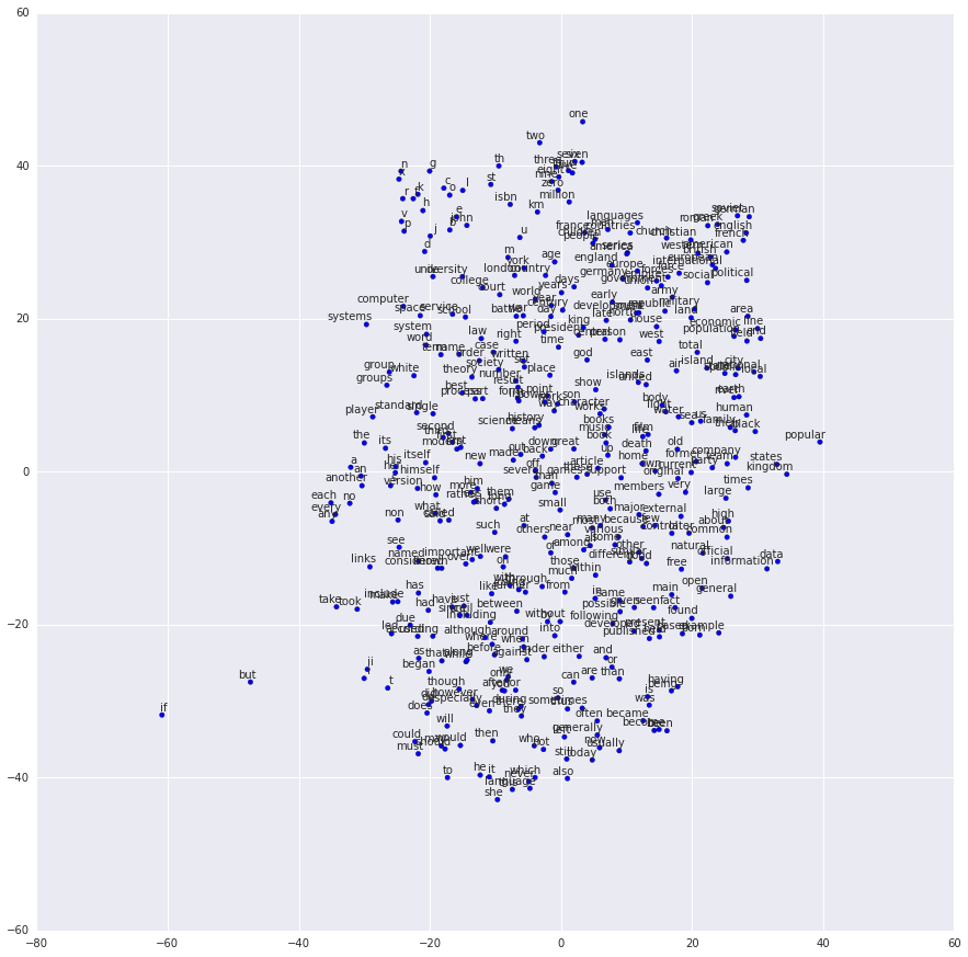
batch_size = 128
embedding_size = 128 # 嵌入向量的维度
skip_window = 1 # 考虑左边和右边多少个词
num_skips = 2 # 复用输入多少次来生成标签
# 我们选取一个随机验证集，来采样最近邻。这里我们将
# 验证样本限制为较低数值 ID 的单词
# 它们的构造也是最频繁的
valid_size = 16 # 单词的随机集合，用于评估相似性
valid_window = 100 # 只选取分布开头的 dev 样本
valid_examples = np.array(random.sample(xrange(valid_window), valid_size))
num_sampled = 64 # 要采样的负样本数量
graph = tf.Graph()
with graph.as_default():
  # 输入数据
  train_dataset = tf.placeholder(tf.int32, shape=[batch_size])
  train_labels = tf.placeholder(tf.int32, shape=[batch_size, 1])
  valid_dataset = tf.constant(valid_examples, dtype=tf.int32)
  # 变量
  embeddings = tf.Variable(
    tf.random_uniform([vocabulary_size, embedding_size], -1.0, 1.0))
  softmax_weights = tf.Variable(
    tf.truncated_normal([vocabulary_size, embedding_size],
                         stddev=1.0 / math.sqrt(embedding_size)))
  softmax_biases = tf.Variable(tf.zeros([vocabulary_size]))
  # 模型
  # Look up embeddings for inputs.
  embed = tf.nn.embedding_lookup(embeddings, train_dataset)
  # Compute the softmax loss, using a sample of the negative labels each time.
  loss = tf.reduce_mean(
    tf.nn.sampled_softmax_loss(softmax_weights, softmax_biases, embed,
                               train_labels, num_sampled, vocabulary_size))
  # 优化器
  optimizer = tf.train.AdagradOptimizer(1.0).minimize(loss)
  # 计算小批量样本和所有嵌入之间的相似性
  # 我们使用余弦距离：
  norm = tf.sqrt(tf.reduce_sum(tf.square(embeddings), 1, keep_dims=True))
  normalized_embeddings = embeddings / norm
  valid_embeddings = tf.nn.embedding_lookup(
    normalized_embeddings, valid_dataset)
  similarity = tf.matmul(valid_embeddings, tf.transpose(normalized_embeddings))
num_steps = 100001
with tf.Session(graph=graph) as session:
  tf.global_variables_initializer().run()
  print "Initialized"
  average_loss = 0
  for step in xrange(num_steps):
    batch_data, batch_labels = generate_batch(
      batch_size, num_skips, skip_window)
    feed_dict = {train_dataset : batch_data, train_labels : batch_labels}
    _, l = session.run([optimizer, loss], feed_dict=feed_dict)
    average_loss += l
    if step % 2000 == 0:
      if step > 0:
        average_loss = average_loss / 2000
      # 平均损失是最后 2000 个批量上的损失的估计
      print "Average loss at step", step, ":", average_loss
      average_loss = 0
    # 注意这非常昂贵（如果计算每 500 步，会慢约 20%）
    if step % 10000 == 0:
      sim = similarity.eval()
      for i in xrange(valid_size):
        valid_word = reverse_dictionary[valid_examples[i]]
        top_k = 8 # 最近邻数量
        nearest = (-sim[i, :]).argsort()[1:top_k+1]
        log = "Nearest to %s:" % valid_word
        for k in xrange(top_k):
          close_word = reverse_dictionary[nearest[k]]
          log = "%s %s," % (log, close_word)
        print log
  final_embeddings = normalized_embeddings.eval()
num_points = 400
tsne = TSNE(perplexity=30, n_components=2, init='pca', n_iter=5000)
two_d_embeddings = tsne.fit_transform(final_embeddings[1:num_points+1, :])
def plot(embeddings, labels):
  assert embeddings.shape[0] >= len(labels), 'More labels than embeddings'
  pylab.figure(figsize=(15,15))  # 以英寸为单位
  for i, label in enumerate(labels):
    x, y = embeddings[i,:]
    pylab.scatter(x, y)
    pylab.annotate(label, xy=(x, y), xytext=(5, 2), textcoords='offset points',
                   ha='right', va='bottom')
  pylab.show()
words = [reverse_dictionary[i] for i in xrange(1, num_points+1)]
plot(two_d_embeddings, words)
'''
Initialized
Average loss at step 0 : 8.58149623871
Nearest to been: unfavourably, marmara, ancestral, legal, bogart, glossaries, worst, rooms,
Nearest to time: conformist, strawberries, sindhi, waterfall, xia, nominates, psp, sensitivity,
Nearest to over: overlord, panda, golden, semigroup, rawlings, involved, shreveport, handling,
Nearest to not: hymenoptera, reintroducing, lamiaceae, because, davao, omnipotent, combustion, debilitating,
Nearest to three: catalog, koza, gn, braque, holstein, postgresql, luddite, justine,
...
Nearest to and: or, but, purview, thirst, sukkot, epr, including, honesty,
Nearest to eight: seven, nine, six, four, five, three, zero, one,
Nearest to they: we, there, you, he, she, prisons, it, these,
Nearest to more: less, most, very, quite, faster, larger, rather, smaller,
Nearest to other: various, different, tamara, theos, some, cope, many, others,
'''

2.6 TensorFlow LSTM

致谢：派生于 Google 的 TensorFlow

配置

参考配置指南.

练习 6

在5_word2vec.ipynb中训练了一个 skip-gram 模型之后，本练习的目标是在 Text8 数据上训练 LSTM 字符模型。

# 这些是我们之后使用的所有模块。 
# 在继续之前，确保你可以导入它们。
import os
import numpy as np
import random
import string
import tensorflow as tf
import urllib
import zipfile
url = 'http://mattmahoney.net/dc/'
def maybe_download(filename, expected_bytes):
  """如果文件不存在则下载，并确保它的大小正确"""
  if not os.path.exists(filename):
    filename, _ = urllib.urlretrieve(url + filename, filename)
  statinfo = os.stat(filename)
  if statinfo.st_size == expected_bytes:
    print 'Found and verified', filename
  else:
    print statinfo.st_size
    raise Exception(
      'Failed to verify ' + filename + '. Can you get to it with a browser?')
  return filename
filename = maybe_download('text8.zip', 31344016)
# Found and verified text8.zip
def read_data(filename):
  f = zipfile.ZipFile(filename)
  for name in f.namelist():
    return f.read(name)
  f.close()
text = read_data(filename)
print "Data size", len(text)
# Data size 100000000

创建一个小型验证集。

valid_size = 1000
valid_text = text[:valid_size]
train_text = text[valid_size:]
train_size = len(train_text)
print train_size, train_text[:64]
print valid_size, valid_text[:64]
'''
99999000 ons anarchists advocate social relations based upon voluntary as
1000  anarchism originated as a term of abuse first used against earl
'''

用于将字符映射到词汇表 ID 并返回的工具。

vocabulary_size = len(string.ascii_lowercase) + 1 # [a-z] + ' '
first_letter = ord(string.ascii_lowercase[0])
def char2id(char):
  if char in string.ascii_lowercase:
    return ord(char) - first_letter + 1
  elif char == ' ':
    return 0
  else:
    print 'Unexpected character:', char
    return 0
def id2char(dictid):
  if dictid > 0:
    return chr(dictid + first_letter - 1)
  else:
    return ' '
print char2id('a'), char2id('z'), char2id(' '), char2id('ï')
print id2char(1), id2char(26), id2char(0)
'''
1 26 0 Unexpected character: ï
0
a z  
'''

用于生成 LSTM 模型的训练批量的函数。

batch_size=64
num_unrollings=10
class BatchGenerator(object):
  def __init__(self, text, batch_size, num_unrollings):
    self._text = text
    self._text_size = len(text)
    self._batch_size = batch_size
    self._num_unrollings = num_unrollings
    segment = self._text_size / batch_size
    self._cursor = [ offset * segment for offset in xrange(batch_size)]
    self._last_batch = self._next_batch()
  def _next_batch(self):
    """从当前游标位置生成单个批量"""
    batch = np.zeros(shape=(self._batch_size, vocabulary_size), dtype=np.float)
    for b in xrange(self._batch_size):
      batch[b, char2id(self._text[self._cursor[b]])] = 1.0
      self._cursor[b] = (self._cursor[b] + 1) % self._text_size
    return batch
  def next(self):
    """从数据中生成批量的下一个数组
    数据包含前一个数组的最后一个批量，后面是 num_unrollings 个新的"""
    batches = [self._last_batch]
    for step in xrange(self._num_unrollings):
      batches.append(self._next_batch())
    self._last_batch = batches[-1]
    return batches
def characters(probabilities):
  """将单热编码，或者可能字符的概率分布转换为它的（最可能的）字符表示"""
  return [id2char(c) for c in np.argmax(probabilities, 1)]
def batches2string(batches):
  """将批量序列转换为它们（最可能的）字符串表示"""
  s = [''] * batches[0].shape[0]
  for b in batches:
    s = [''.join(x) for x in zip(s, characters(b))]
  return s
train_batches = BatchGenerator(train_text, batch_size, num_unrollings)
valid_batches = BatchGenerator(valid_text, 1, 1)
print batches2string(train_batches.next())
print batches2string(train_batches.next())
print batches2string(valid_batches.next())
print batches2string(valid_batches.next())
'''
['ons anarchi', 'when milita', 'lleria arch', ' abbeys and', 'married urr', 'hel and ric', 'y and litur', 'ay opened f', 'tion from t', 'migration t', 'new york ot', 'he boeing s', 'e listed wi', 'eber has pr', 'o be made t', 'yer who rec', 'ore signifi', 'a fierce cr', ' two six ei', 'aristotle s', 'ity can be ', ' and intrac', 'tion of the', 'dy to pass ', 'f certain d', 'at it will ', 'e convince ', 'ent told hi', 'ampaign and', 'rver side s', 'ious texts ', 'o capitaliz', 'a duplicate', 'gh ann es d', 'ine january', 'ross zero t', 'cal theorie', 'ast instanc', ' dimensiona', 'most holy m', 't s support', 'u is still ', 'e oscillati', 'o eight sub', 'of italy la', 's the tower', 'klahoma pre', 'erprise lin', 'ws becomes ', 'et in a naz', 'the fabian ', 'etchy to re', ' sharman ne', 'ised empero', 'ting in pol', 'd neo latin', 'th risky ri', 'encyclopedi', 'fense the a', 'duating fro', 'treet grid ', 'ations more', 'appeal of d', 'si have mad']
['ists advoca', 'ary governm', 'hes nationa', 'd monasteri', 'raca prince', 'chard baer ', 'rgical lang', 'for passeng', 'the nationa', 'took place ', 'ther well k', 'seven six s', 'ith a gloss', 'robably bee', 'to recogniz', 'ceived the ', 'icant than ', 'ritic of th', 'ight in sig', 's uncaused ', ' lost as in', 'cellular ic', 'e size of t', ' him a stic', 'drugs confu', ' take to co', ' the priest', 'im to name ', 'd barred at', 'standard fo', ' such as es', 'ze on the g', 'e of the or', 'd hiver one', 'y eight mar', 'the lead ch', 'es classica', 'ce the non ', 'al analysis', 'mormons bel', 't or at lea', ' disagreed ', 'ing system ', 'btypes base', 'anguages th', 'r commissio', 'ess one nin', 'nux suse li', ' the first ', 'zi concentr', ' society ne', 'elatively s', 'etworks sha', 'or hirohito', 'litical ini', 'n most of t', 'iskerdoo ri', 'ic overview', 'air compone', 'om acnm acc', ' centerline', 'e than any ', 'devotional ', 'de such dev']
[' a']
['an']
'''
def logprob(predictions, labels):
  """预测批量中的真实标签的对数概率"""
  predictions[predictions < 1e-10] = 1e-10
  return np.sum(np.multiply(labels, -np.log(predictions))) / labels.shape[0]
def sample_distribution(distribution):
  """从分布中抽取一个元素，分布假设为标准化概率的数组  """
  r = random.uniform(0, 1)
  s = 0
  for i in xrange(len(distribution)):
    s += distribution[i]
    if s >= r:
      return i
  return len(distribution) - 1
def sample(prediction):
  """将一列预测转换为单热编码的样本"""
  p = np.zeros(shape=[1, vocabulary_size], dtype=np.float)
  p[0, sample_distribution(prediction[0])] = 1.0
  return p
def random_distribution():
  """生成概率的随机列"""
  b = np.random.uniform(0.0, 1.0, size=[1, vocabulary_size])
  return b/np.sum(b, 1)[:,None]