译者:飞龙
1.1 TensorFlow 基本操作
致谢:派生于 Aymeric Damien 的 TensorFlow 示例
配置
参考配置指南。
import tensorflow as tf# 基本的常量操作# 由构造器返回的值# 表示常量操作的输出a = tf.constant(2)b = tf.constant(3)# 加载默认图with tf.Session() as sess:print "a=2, b=3"print "Addition with constants: %i" % sess.run(a+b)print "Multiplication with constants: %i" % sess.run(a*b)'''a=2, b=3Addition with constants: 5Multiplication with constants: 6'''# 作为图输入的变量的基本操作# 由构造器返回的值# 表示变量操作的输出(运行会话时定义为输出)# TF 图输入a = tf.placeholder(tf.int16)b = tf.placeholder(tf.int16)# 定义一些操作add = tf.add(a, b)mul = tf.mul(a, b)# 加载默认图with tf.Session() as sess:# 使用遍历输入运行每个操作print "Addition with variables: %i" % sess.run(add, feed_dict={a: 2, b: 3})print "Multiplication with variables: %i" % sess.run(mul, feed_dict={a: 2, b: 3})'''Addition with variables: 5Multiplication with variables: 6'''# ----------------# 更多细节:# 来自 TF 官方教程的矩阵乘法教程# 创建常量操作,产生 1x2 矩阵# 操作作为节点添加到默认图中## 由构造器返回的值# 表示常量操作的输出matrix1 = tf.constant([[3., 3.]])# 创建另一个常量,产生 2x1 矩阵matrix2 = tf.constant([[2.],[2.]])# 创建 Matmul 操作,它接受 'matrix1' 和 'matrix2' 作为输入# 返回的值 'product' 表示矩阵乘法的结果product = tf.matmul(matrix1, matrix2)# 为了执行 matmul 操作,我们调用会话的 'run()' 方法,传入 'product'# 它表示 matmul 操作的输出。这对调用表明我们向获取 matmul 操作的输出## 操作所需的所有输入都由会话自动运行# 它们通常是并行运行的## 'run(product)' 的调用会执行图中的三个操作:# 两个常量和 matmul## 操作的输出在 'result' 中返回,作为 NumPy `ndarray` 对象with tf.Session() as sess:result = sess.run(product)print result# [[ 12.]]
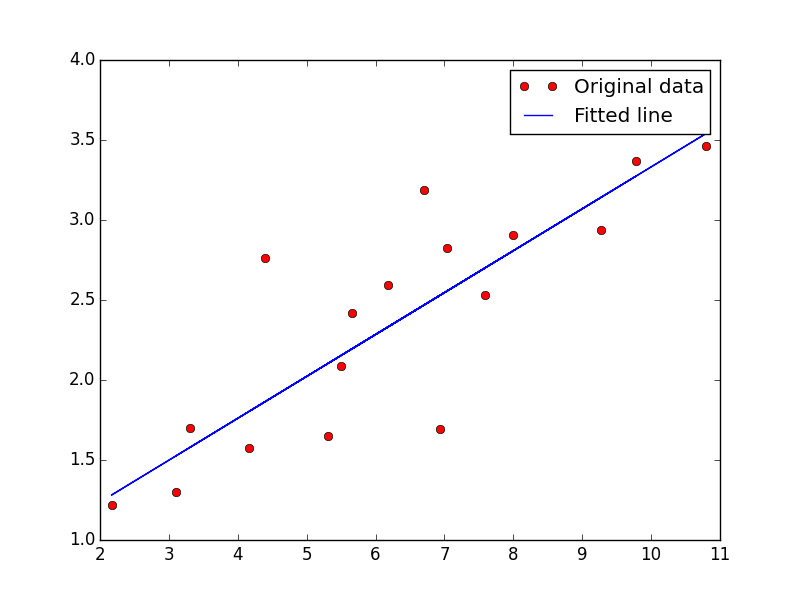
1.2 TensorFlow 线性回归
致谢:派生于 Aymeric Damien 的 TensorFlow 示例
配置
参考配置指南。
import tensorflow as tfimport numpyimport matplotlib.pyplot as pltrng = numpy.random# 参数learning_rate = 0.01training_epochs = 2000display_step = 50# 训练数据train_X = numpy.asarray([3.3,4.4,5.5,6.71,6.93,4.168,9.779,6.182,7.59,2.167,7.042,10.791,5.313,7.997,5.654,9.27,3.1])train_Y = numpy.asarray([1.7,2.76,2.09,3.19,1.694,1.573,3.366,2.596,2.53,1.221,2.827,3.465,1.65,2.904,2.42,2.94,1.3])n_samples = train_X.shape[0]# TF 图输入X = tf.placeholder("float")Y = tf.placeholder("float")# 创建模型# 设置模型权重W = tf.Variable(rng.randn(), name="weight")b = tf.Variable(rng.randn(), name="bias")# 构造线性模型activation = tf.add(tf.mul(X, W), b)# 最小化平方误差cost = tf.reduce_sum(tf.pow(activation-Y, 2))/(2*n_samples) #L2 lossoptimizer = tf.train.GradientDescentOptimizer(learning_rate).minimize(cost) #Gradient descent# 初始化变量init = tf.initialize_all_variables()# 加载图with tf.Session() as sess:sess.run(init)# 拟合所有训练数据for epoch in range(training_epochs):for (x, y) in zip(train_X, train_Y):sess.run(optimizer, feed_dict={X: x, Y: y})# 展示每一步的日志if epoch % display_step == 0:print "Epoch:", '%04d' % (epoch+1), "cost=", \"{:.9f}".format(sess.run(cost, feed_dict={X: train_X, Y:train_Y})), \"W=", sess.run(W), "b=", sess.run(b)print "Optimization Finished!"print "cost=", sess.run(cost, feed_dict={X: train_X, Y: train_Y}), \"W=", sess.run(W), "b=", sess.run(b)# 展示图plt.plot(train_X, train_Y, 'ro', label='Original data')plt.plot(train_X, sess.run(W) * train_X + sess.run(b), label='Fitted line')plt.legend()plt.show()'''Epoch: 0001 cost= 3.389688730 W= 0.0198441 b= -0.273522Epoch: 0051 cost= 0.134034902 W= 0.383208 b= -0.159746Epoch: 0101 cost= 0.127440125 W= 0.375261 b= -0.102578Epoch: 0151 cost= 0.121607177 W= 0.367787 b= -0.0488099Epoch: 0201 cost= 0.116448022 W= 0.360758 b= 0.00175997Epoch: 0251 cost= 0.111884907 W= 0.354146 b= 0.0493223Epoch: 0301 cost= 0.107848980 W= 0.347928 b= 0.0940558Epoch: 0351 cost= 0.104279339 W= 0.34208 b= 0.136129Epoch: 0401 cost= 0.101122171 W= 0.336579 b= 0.1757Epoch: 0451 cost= 0.098329842 W= 0.331405 b= 0.212917Epoch: 0501 cost= 0.095860250 W= 0.32654 b= 0.247921Epoch: 0551 cost= 0.093676031 W= 0.321963 b= 0.280843Epoch: 0601 cost= 0.091744311 W= 0.317659 b= 0.311807Epoch: 0651 cost= 0.090035893 W= 0.313611 b= 0.340929Epoch: 0701 cost= 0.088524953 W= 0.309804 b= 0.36832Epoch: 0751 cost= 0.087188691 W= 0.306222 b= 0.394082Epoch: 0801 cost= 0.086007021 W= 0.302854 b= 0.418311Epoch: 0851 cost= 0.084961981 W= 0.299687 b= 0.441099Epoch: 0901 cost= 0.084037818 W= 0.296708 b= 0.462532Epoch: 0951 cost= 0.083220571 W= 0.293905 b= 0.48269Epoch: 1001 cost= 0.082497880 W= 0.29127 b= 0.50165Epoch: 1051 cost= 0.081858821 W= 0.288791 b= 0.519481Epoch: 1101 cost= 0.081293717 W= 0.28646 b= 0.536251Epoch: 1151 cost= 0.080794014 W= 0.284267 b= 0.552026Epoch: 1201 cost= 0.080352172 W= 0.282205 b= 0.566861Epoch: 1251 cost= 0.079961479 W= 0.280265 b= 0.580815Epoch: 1301 cost= 0.079616025 W= 0.278441 b= 0.593939Epoch: 1351 cost= 0.079310589 W= 0.276725 b= 0.606284Epoch: 1401 cost= 0.079040587 W= 0.275111 b= 0.617893Epoch: 1451 cost= 0.078801893 W= 0.273594 b= 0.62881Epoch: 1501 cost= 0.078590907 W= 0.272167 b= 0.639077Epoch: 1551 cost= 0.078404360 W= 0.270824 b= 0.648734Epoch: 1601 cost= 0.078239456 W= 0.269562 b= 0.657817Epoch: 1651 cost= 0.078093678 W= 0.268374 b= 0.66636Epoch: 1701 cost= 0.077964827 W= 0.267257 b= 0.674395Epoch: 1751 cost= 0.077850945 W= 0.266207 b= 0.681952Epoch: 1801 cost= 0.077750273 W= 0.265219 b= 0.68906Epoch: 1851 cost= 0.077661335 W= 0.264289 b= 0.695745Epoch: 1901 cost= 0.077582702 W= 0.263416 b= 0.702033Epoch: 1951 cost= 0.077513263 W= 0.262593 b= 0.707947Optimization Finished!cost= 0.077453 W= 0.261835 b= 0.713401'''from IPython.display import ImageImage(filename='linearreg.png')
1.3 TensorFlow Logistic 回归
致谢:派生于 Aymeric Damien 的 TensorFlow 示例
配置
参考配置指南。
# 导入 MINST 数据import input_datamnist = input_data.read_data_sets("/tmp/data/", one_hot=True)'''Extracting /tmp/data/train-images-idx3-ubyte.gzExtracting /tmp/data/train-labels-idx1-ubyte.gzExtracting /tmp/data/t10k-images-idx3-ubyte.gzExtracting /tmp/data/t10k-labels-idx1-ubyte.gz'''import tensorflow as tf# 参数learning_rate = 0.01training_epochs = 25batch_size = 100display_step = 1# TF 图输入x = tf.placeholder("float", [None, 784]) # mnist 数据图像,形状为 28*28=784y = tf.placeholder("float", [None, 10]) # 0-9 数字识别 => 10 个类# 创建模型# 设置模型权重W = tf.Variable(tf.zeros([784, 10]))b = tf.Variable(tf.zeros([10]))# 构造模型activation = tf.nn.softmax(tf.matmul(x, W) + b) # Softmax# 最小化交叉熵误差# 交叉熵cost = -tf.reduce_sum(y*tf.log(activation))# 梯度下降optimizer = tf.train.GradientDescentOptimizer(learning_rate).minimize(cost)# 初始化变量init = tf.initialize_all_variables()# 加载图with tf.Session() as sess:sess.run(init)# 训练循环for epoch in range(training_epochs):avg_cost = 0.total_batch = int(mnist.train.num_examples/batch_size)# 遍历所有批量for i in range(total_batch):batch_xs, batch_ys = mnist.train.next_batch(batch_size)# 使用批量数据拟合训练sess.run(optimizer, feed_dict={x: batch_xs, y: batch_ys})# 计算平均损失avg_cost += sess.run(cost, feed_dict={x: batch_xs, y: batch_ys})/total_batch# 展示每一步的日志if epoch % display_step == 0:print "Epoch:", '%04d' % (epoch+1), "cost=", "{:.9f}".format(avg_cost)print "Optimization Finished!"# 测试模型correct_prediction = tf.equal(tf.argmax(activation, 1), tf.argmax(y, 1))# 计算准确率accuracy = tf.reduce_mean(tf.cast(correct_prediction, "float"))print "Accuracy:", accuracy.eval({x: mnist.test.images, y: mnist.test.labels})'''Epoch: 0001 cost= 29.860479714Epoch: 0002 cost= 22.080549484Epoch: 0003 cost= 21.237104595Epoch: 0004 cost= 20.460196280Epoch: 0005 cost= 20.185128237Epoch: 0006 cost= 19.940297202Epoch: 0007 cost= 19.645111119Epoch: 0008 cost= 19.507218031Epoch: 0009 cost= 19.389794492Epoch: 0010 cost= 19.177005816Epoch: 0011 cost= 19.082493615Epoch: 0012 cost= 19.072873598Epoch: 0013 cost= 18.938005402Epoch: 0014 cost= 18.891806430Epoch: 0015 cost= 18.839480221Epoch: 0016 cost= 18.769349510Epoch: 0017 cost= 18.590865587Epoch: 0018 cost= 18.623413677Epoch: 0019 cost= 18.546149085Epoch: 0020 cost= 18.432274895Epoch: 0021 cost= 18.358189004Epoch: 0022 cost= 18.380014628Epoch: 0023 cost= 18.499993471Epoch: 0024 cost= 18.386477311Epoch: 0025 cost= 18.258080609Optimization Finished!Accuracy: 0.9048'''
1.4 TensorFlow 最近邻
致谢:派生于 Aymeric Damien 的 TensorFlow 示例
配置
参考配置指南。
import numpy as npimport tensorflow as tf# 导入 MINST 数据import input_datamnist = input_data.read_data_sets("/tmp/data/", one_hot=True)'''Extracting /tmp/data/train-images-idx3-ubyte.gzExtracting /tmp/data/train-labels-idx1-ubyte.gzExtracting /tmp/data/t10k-images-idx3-ubyte.gzExtracting /tmp/data/t10k-labels-idx1-ubyte.gz'''# 这个例子中,我们限制 mnist 数据Xtr, Ytr = mnist.train.next_batch(5000) # 训练集 5000 个(nn 候选)Xte, Yte = mnist.test.next_batch(200) # 测试集 200 个# 将图像的形状变为一维Xtr = np.reshape(Xtr, newshape=(-1, 28*28))Xte = np.reshape(Xte, newshape=(-1, 28*28))# TF 图输入xtr = tf.placeholder("float", [None, 784])xte = tf.placeholder("float", [784])# 使用 L1 距离计算最近邻distance = tf.reduce_sum(tf.abs(tf.add(xtr, tf.neg(xte))), reduction_indices=1)# 预测:获取最小距离的下标(最近邻)pred = tf.arg_min(distance, 0)accuracy = 0.# 初始化变量init = tf.initialize_all_variables()# 加载图with tf.Session() as sess:sess.run(init)# 遍历测试数据for i in range(len(Xte)):# 获取最近邻nn_index = sess.run(pred, feed_dict={xtr: Xtr, xte: Xte[i,:]})# 获取最近邻的类标签,并将其与真实标签比较print "Test", i, "Prediction:", np.argmax(Ytr[nn_index]), \"True Class:", np.argmax(Yte[i])# 计算准确率if np.argmax(Ytr[nn_index]) == np.argmax(Yte[i]):accuracy += 1./len(Xte)print "Done!"print "Accuracy:", accuracy'''Test 0 Prediction: 7 True Class: 7Test 1 Prediction: 2 True Class: 2Test 2 Prediction: 1 True Class: 1Test 3 Prediction: 0 True Class: 0Test 4 Prediction: 4 True Class: 4Test 5 Prediction: 1 True Class: 1Test 6 Prediction: 4 True Class: 4Test 7 Prediction: 9 True Class: 9Test 8 Prediction: 8 True Class: 5Test 9 Prediction: 9 True Class: 9Test 10 Prediction: 0 True Class: 0Test 11 Prediction: 0 True Class: 6Test 12 Prediction: 9 True Class: 9Test 13 Prediction: 0 True Class: 0Test 14 Prediction: 1 True Class: 1Test 15 Prediction: 5 True Class: 5Test 16 Prediction: 4 True Class: 9Test 17 Prediction: 7 True Class: 7Test 18 Prediction: 3 True Class: 3Test 19 Prediction: 4 True Class: 4Test 20 Prediction: 9 True Class: 9Test 21 Prediction: 6 True Class: 6Test 22 Prediction: 6 True Class: 6Test 23 Prediction: 5 True Class: 5Test 24 Prediction: 4 True Class: 4Test 25 Prediction: 0 True Class: 0Test 26 Prediction: 7 True Class: 7Test 27 Prediction: 4 True Class: 4Test 28 Prediction: 0 True Class: 0Test 29 Prediction: 1 True Class: 1Test 30 Prediction: 3 True Class: 3Test 31 Prediction: 1 True Class: 1Test 32 Prediction: 3 True Class: 3Test 33 Prediction: 4 True Class: 4Test 34 Prediction: 7 True Class: 7Test 35 Prediction: 2 True Class: 2Test 36 Prediction: 7 True Class: 7Test 37 Prediction: 1 True Class: 1Test 38 Prediction: 2 True Class: 2Test 39 Prediction: 1 True Class: 1Test 40 Prediction: 1 True Class: 1Test 41 Prediction: 7 True Class: 7Test 42 Prediction: 4 True Class: 4Test 43 Prediction: 1 True Class: 2Test 44 Prediction: 3 True Class: 3Test 45 Prediction: 5 True Class: 5Test 46 Prediction: 1 True Class: 1Test 47 Prediction: 2 True Class: 2Test 48 Prediction: 4 True Class: 4Test 49 Prediction: 4 True Class: 4Test 50 Prediction: 6 True Class: 6Test 51 Prediction: 3 True Class: 3Test 52 Prediction: 5 True Class: 5Test 53 Prediction: 5 True Class: 5Test 54 Prediction: 6 True Class: 6Test 55 Prediction: 0 True Class: 0Test 56 Prediction: 4 True Class: 4Test 57 Prediction: 1 True Class: 1Test 58 Prediction: 9 True Class: 9Test 59 Prediction: 5 True Class: 5Test 60 Prediction: 7 True Class: 7Test 61 Prediction: 8 True Class: 8Test 62 Prediction: 9 True Class: 9Test 63 Prediction: 3 True Class: 3Test 64 Prediction: 7 True Class: 7Test 65 Prediction: 4 True Class: 4Test 66 Prediction: 6 True Class: 6Test 67 Prediction: 4 True Class: 4Test 68 Prediction: 3 True Class: 3Test 69 Prediction: 0 True Class: 0Test 70 Prediction: 7 True Class: 7Test 71 Prediction: 0 True Class: 0Test 72 Prediction: 2 True Class: 2Test 73 Prediction: 7 True Class: 9Test 74 Prediction: 1 True Class: 1Test 75 Prediction: 7 True Class: 7Test 76 Prediction: 3 True Class: 3Test 77 Prediction: 7 True Class: 2Test 78 Prediction: 9 True Class: 9Test 79 Prediction: 7 True Class: 7Test 80 Prediction: 7 True Class: 7Test 81 Prediction: 6 True Class: 6Test 82 Prediction: 2 True Class: 2Test 83 Prediction: 7 True Class: 7Test 84 Prediction: 8 True Class: 8Test 85 Prediction: 4 True Class: 4Test 86 Prediction: 7 True Class: 7Test 87 Prediction: 3 True Class: 3Test 88 Prediction: 6 True Class: 6Test 89 Prediction: 1 True Class: 1Test 90 Prediction: 3 True Class: 3Test 91 Prediction: 6 True Class: 6Test 92 Prediction: 9 True Class: 9Test 93 Prediction: 3 True Class: 3Test 94 Prediction: 1 True Class: 1Test 95 Prediction: 4 True Class: 4Test 96 Prediction: 1 True Class: 1Test 97 Prediction: 7 True Class: 7Test 98 Prediction: 6 True Class: 6Test 99 Prediction: 9 True Class: 9Test 100 Prediction: 6 True Class: 6Test 101 Prediction: 0 True Class: 0Test 102 Prediction: 5 True Class: 5Test 103 Prediction: 4 True Class: 4Test 104 Prediction: 9 True Class: 9Test 105 Prediction: 9 True Class: 9Test 106 Prediction: 2 True Class: 2Test 107 Prediction: 1 True Class: 1Test 108 Prediction: 9 True Class: 9Test 109 Prediction: 4 True Class: 4Test 110 Prediction: 8 True Class: 8Test 111 Prediction: 7 True Class: 7Test 112 Prediction: 3 True Class: 3Test 113 Prediction: 9 True Class: 9Test 114 Prediction: 7 True Class: 7Test 115 Prediction: 9 True Class: 4Test 116 Prediction: 9 True Class: 4Test 117 Prediction: 4 True Class: 4Test 118 Prediction: 9 True Class: 9Test 119 Prediction: 7 True Class: 2Test 120 Prediction: 5 True Class: 5Test 121 Prediction: 4 True Class: 4Test 122 Prediction: 7 True Class: 7Test 123 Prediction: 6 True Class: 6Test 124 Prediction: 7 True Class: 7Test 125 Prediction: 9 True Class: 9Test 126 Prediction: 0 True Class: 0Test 127 Prediction: 5 True Class: 5Test 128 Prediction: 8 True Class: 8Test 129 Prediction: 5 True Class: 5Test 130 Prediction: 6 True Class: 6Test 131 Prediction: 6 True Class: 6Test 132 Prediction: 5 True Class: 5Test 133 Prediction: 7 True Class: 7Test 134 Prediction: 8 True Class: 8Test 135 Prediction: 1 True Class: 1Test 136 Prediction: 0 True Class: 0Test 137 Prediction: 1 True Class: 1Test 138 Prediction: 6 True Class: 6Test 139 Prediction: 4 True Class: 4Test 140 Prediction: 6 True Class: 6Test 141 Prediction: 7 True Class: 7Test 142 Prediction: 2 True Class: 3Test 143 Prediction: 1 True Class: 1Test 144 Prediction: 7 True Class: 7Test 145 Prediction: 1 True Class: 1Test 146 Prediction: 8 True Class: 8Test 147 Prediction: 2 True Class: 2Test 148 Prediction: 0 True Class: 0Test 149 Prediction: 1 True Class: 2Test 150 Prediction: 9 True Class: 9Test 151 Prediction: 9 True Class: 9Test 152 Prediction: 5 True Class: 5Test 153 Prediction: 5 True Class: 5Test 154 Prediction: 1 True Class: 1Test 155 Prediction: 5 True Class: 5Test 156 Prediction: 6 True Class: 6Test 157 Prediction: 0 True Class: 0Test 158 Prediction: 3 True Class: 3Test 159 Prediction: 4 True Class: 4Test 160 Prediction: 4 True Class: 4Test 161 Prediction: 6 True Class: 6Test 162 Prediction: 5 True Class: 5Test 163 Prediction: 4 True Class: 4Test 164 Prediction: 6 True Class: 6Test 165 Prediction: 5 True Class: 5Test 166 Prediction: 4 True Class: 4Test 167 Prediction: 5 True Class: 5Test 168 Prediction: 1 True Class: 1Test 169 Prediction: 4 True Class: 4Test 170 Prediction: 9 True Class: 4Test 171 Prediction: 7 True Class: 7Test 172 Prediction: 2 True Class: 2Test 173 Prediction: 3 True Class: 3Test 174 Prediction: 2 True Class: 2Test 175 Prediction: 1 True Class: 7Test 176 Prediction: 1 True Class: 1Test 177 Prediction: 8 True Class: 8Test 178 Prediction: 1 True Class: 1Test 179 Prediction: 8 True Class: 8Test 180 Prediction: 1 True Class: 1Test 181 Prediction: 8 True Class: 8Test 182 Prediction: 5 True Class: 5Test 183 Prediction: 0 True Class: 0Test 184 Prediction: 2 True Class: 8Test 185 Prediction: 9 True Class: 9Test 186 Prediction: 2 True Class: 2Test 187 Prediction: 5 True Class: 5Test 188 Prediction: 0 True Class: 0Test 189 Prediction: 1 True Class: 1Test 190 Prediction: 1 True Class: 1Test 191 Prediction: 1 True Class: 1Test 192 Prediction: 0 True Class: 0Test 193 Prediction: 4 True Class: 9Test 194 Prediction: 0 True Class: 0Test 195 Prediction: 1 True Class: 3Test 196 Prediction: 1 True Class: 1Test 197 Prediction: 6 True Class: 6Test 198 Prediction: 4 True Class: 4Test 199 Prediction: 2 True Class: 2Done!Accuracy: 0.92'''
1.5 TensorFlow AlexNet
致谢:派生于 Aymeric Damien 的 TensorFlow 示例
配置
参考配置指南。
# 导入 MINST 数据import input_datamnist = input_data.read_data_sets("/tmp/data/", one_hot=True)'''Extracting /tmp/data/train-images-idx3-ubyte.gzExtracting /tmp/data/train-labels-idx1-ubyte.gzExtracting /tmp/data/t10k-images-idx3-ubyte.gzExtracting /tmp/data/t10k-labels-idx1-ubyte.gz'''import tensorflow as tf# 参数learning_rate = 0.001training_iters = 300000batch_size = 64display_step = 100# 网络参数n_input = 784 # MNIST 数据输入(图像大小:28x28)n_classes = 10 # MNIST 全部类别(0-9 的数字)dropout = 0.8 # 丢弃,单元被保留的概率# TF 图输入x = tf.placeholder(tf.float32, [None, n_input])y = tf.placeholder(tf.float32, [None, n_classes])keep_prob = tf.placeholder(tf.float32) # 丢弃(保留的概率)# 创建 AlexNet 模型def conv2d(name, l_input, w, b):return tf.nn.relu(tf.nn.bias_add(tf.nn.conv2d(l_input, w, strides=[1, 1, 1, 1],padding='SAME'),b), name=name)def max_pool(name, l_input, k):return tf.nn.max_pool(l_input, ksize=[1, k, k, 1], strides=[1, k, k, 1],padding='SAME', name=name)def norm(name, l_input, lsize=4):return tf.nn.lrn(l_input, lsize, bias=1.0, alpha=0.001 / 9.0, beta=0.75, name=name)def alex_net(_X, _weights, _biases, _dropout):# 改变输入图片的形状_X = tf.reshape(_X, shape=[-1, 28, 28, 1])# 卷积层conv1 = conv2d('conv1', _X, _weights['wc1'], _biases['bc1'])# 最大池化(下采样)pool1 = max_pool('pool1', conv1, k=2)# 应用标准化norm1 = norm('norm1', pool1, lsize=4)# 应用丢弃norm1 = tf.nn.dropout(norm1, _dropout)# 卷积层conv2 = conv2d('conv2', norm1, _weights['wc2'], _biases['bc2'])# 最大池化(下采样)pool2 = max_pool('pool2', conv2, k=2)# 应用标准化norm2 = norm('norm2', pool2, lsize=4)# 应用丢弃norm2 = tf.nn.dropout(norm2, _dropout)# 卷积层conv3 = conv2d('conv3', norm2, _weights['wc3'], _biases['bc3'])# 最大池化(下采样)pool3 = max_pool('pool3', conv3, k=2)# 应用标准化norm3 = norm('norm3', pool3, lsize=4)# 应用丢弃norm3 = tf.nn.dropout(norm3, _dropout)# 全连接层# 修改 conv3 输出的形状来匹配密集层的输入dense1 = tf.reshape(norm3, [-1, _weights['wd1'].get_shape().as_list()[0]])# Relu 激活dense1 = tf.nn.relu(tf.matmul(dense1, _weights['wd1']) + _biases['bd1'], name='fc1')# Relu 激活dense2 = tf.nn.relu(tf.matmul(dense1, _weights['wd2']) + _biases['bd2'], name='fc2')# 输出,类的预测out = tf.matmul(dense2, _weights['out']) + _biases['out']return out# 储存层的权重和偏置weights = {'wc1': tf.Variable(tf.random_normal([3, 3, 1, 64])),'wc2': tf.Variable(tf.random_normal([3, 3, 64, 128])),'wc3': tf.Variable(tf.random_normal([3, 3, 128, 256])),'wd1': tf.Variable(tf.random_normal([4*4*256, 1024])),'wd2': tf.Variable(tf.random_normal([1024, 1024])),'out': tf.Variable(tf.random_normal([1024, 10]))}biases = {'bc1': tf.Variable(tf.random_normal([64])),'bc2': tf.Variable(tf.random_normal([128])),'bc3': tf.Variable(tf.random_normal([256])),'bd1': tf.Variable(tf.random_normal([1024])),'bd2': tf.Variable(tf.random_normal([1024])),'out': tf.Variable(tf.random_normal([n_classes]))}# 构造模型pred = alex_net(x, weights, biases, keep_prob)# 定义损失和优化器cost = tf.reduce_mean(tf.nn.softmax_cross_entropy_with_logits(pred, y))optimizer = tf.train.AdamOptimizer(learning_rate=learning_rate).minimize(cost)# 评估模型correct_pred = tf.equal(tf.argmax(pred,1), tf.argmax(y,1))accuracy = tf.reduce_mean(tf.cast(correct_pred, tf.float32))# 初始化变量init = tf.global_variables_initializer()# 加载图with tf.Session() as sess:sess.run(init)step = 1# 持续训练,直到达到最大迭代while step * batch_size < training_iters:batch_xs, batch_ys = mnist.train.next_batch(batch_size)# 使用批量数据拟合训练sess.run(optimizer, feed_dict={x: batch_xs, y: batch_ys, keep_prob: dropout})if step % display_step == 0:# 计算批量准确率acc = sess.run(accuracy, feed_dict={x: batch_xs, y: batch_ys, keep_prob: 1.})# 计算批量损失loss = sess.run(cost, feed_dict={x: batch_xs, y: batch_ys, keep_prob: 1.})print "Iter " + str(step*batch_size) + ", Minibatch Loss= " \+ "{:.6f}".format(loss) + ", Training Accuracy= " + "{:.5f}".format(acc)step += 1print "Optimization Finished!"# 为 256 个 mnist 测试图像计算准确率print "Testing Accuracy:", sess.run(accuracy, feed_dict={x: mnist.test.images[:256],y: mnist.test.labels[:256],keep_prob: 1.})'''Iter 6400, Minibatch Loss= 29666.185547, Training Accuracy= 0.59375Iter 12800, Minibatch Loss= 22125.562500, Training Accuracy= 0.60938Iter 19200, Minibatch Loss= 22631.134766, Training Accuracy= 0.59375Iter 25600, Minibatch Loss= 18498.414062, Training Accuracy= 0.62500Iter 32000, Minibatch Loss= 11318.283203, Training Accuracy= 0.70312Iter 38400, Minibatch Loss= 12076.280273, Training Accuracy= 0.70312Iter 44800, Minibatch Loss= 8195.520508, Training Accuracy= 0.82812Iter 51200, Minibatch Loss= 5176.181641, Training Accuracy= 0.84375Iter 57600, Minibatch Loss= 8951.896484, Training Accuracy= 0.81250Iter 64000, Minibatch Loss= 10096.946289, Training Accuracy= 0.78125Iter 70400, Minibatch Loss= 11466.641602, Training Accuracy= 0.68750Iter 76800, Minibatch Loss= 7469.824219, Training Accuracy= 0.78125Iter 83200, Minibatch Loss= 4147.449219, Training Accuracy= 0.89062Iter 89600, Minibatch Loss= 5904.782227, Training Accuracy= 0.82812Iter 96000, Minibatch Loss= 718.493713, Training Accuracy= 0.93750Iter 102400, Minibatch Loss= 2184.151367, Training Accuracy= 0.93750Iter 108800, Minibatch Loss= 2354.463135, Training Accuracy= 0.89062Iter 115200, Minibatch Loss= 8612.959961, Training Accuracy= 0.81250Iter 121600, Minibatch Loss= 2225.773926, Training Accuracy= 0.84375Iter 128000, Minibatch Loss= 160.583618, Training Accuracy= 0.96875Iter 134400, Minibatch Loss= 1524.846069, Training Accuracy= 0.93750Iter 140800, Minibatch Loss= 3501.871094, Training Accuracy= 0.89062Iter 147200, Minibatch Loss= 661.977051, Training Accuracy= 0.96875Iter 153600, Minibatch Loss= 367.857788, Training Accuracy= 0.98438Iter 160000, Minibatch Loss= 1735.458740, Training Accuracy= 0.90625Iter 166400, Minibatch Loss= 209.320374, Training Accuracy= 0.95312Iter 172800, Minibatch Loss= 1788.553955, Training Accuracy= 0.90625Iter 179200, Minibatch Loss= 912.995544, Training Accuracy= 0.93750Iter 185600, Minibatch Loss= 2534.074463, Training Accuracy= 0.87500Iter 192000, Minibatch Loss= 73.052612, Training Accuracy= 0.96875Iter 198400, Minibatch Loss= 1609.606323, Training Accuracy= 0.93750Iter 204800, Minibatch Loss= 1823.219727, Training Accuracy= 0.96875Iter 211200, Minibatch Loss= 578.051086, Training Accuracy= 0.96875Iter 217600, Minibatch Loss= 1532.326172, Training Accuracy= 0.89062Iter 224000, Minibatch Loss= 769.775269, Training Accuracy= 0.95312Iter 230400, Minibatch Loss= 2614.737793, Training Accuracy= 0.92188Iter 236800, Minibatch Loss= 938.664368, Training Accuracy= 0.95312Iter 243200, Minibatch Loss= 1520.495605, Training Accuracy= 0.93750Iter 249600, Minibatch Loss= 657.419739, Training Accuracy= 0.95312Iter 256000, Minibatch Loss= 522.802124, Training Accuracy= 0.90625Iter 262400, Minibatch Loss= 211.188477, Training Accuracy= 0.96875Iter 268800, Minibatch Loss= 520.451172, Training Accuracy= 0.92188Iter 275200, Minibatch Loss= 1418.759155, Training Accuracy= 0.89062Iter 281600, Minibatch Loss= 241.748596, Training Accuracy= 0.96875Iter 288000, Minibatch Loss= 0.000000, Training Accuracy= 1.00000Iter 294400, Minibatch Loss= 1535.772827, Training Accuracy= 0.92188Optimization Finished!Testing Accuracy: 0.980469'''
1.6 TensorFlow 卷积神经网络
致谢:派生于 Aymeric Damien 的 TensorFlow 示例
配置
参考配置指南。
# 导入 MINST 数据import input_datamnist = input_data.read_data_sets("/tmp/data/", one_hot=True)'''Extracting /tmp/data/train-images-idx3-ubyte.gzExtracting /tmp/data/train-labels-idx1-ubyte.gzExtracting /tmp/data/t10k-images-idx3-ubyte.gzExtracting /tmp/data/t10k-labels-idx1-ubyte.gz'''import tensorflow as tf# 参数learning_rate = 0.001training_iters = 100000batch_size = 128display_step = 20# 网络参数n_input = 784 # MNIST 数据输入(图像大小:28x28)n_classes = 10 # MNIST 全部类别(0-9 的数字)dropout = 0.75 # 丢弃,单元被保留的概率# TF 图输入x = tf.placeholder(tf.float32, [None, n_input])y = tf.placeholder(tf.float32, [None, n_classes])keep_prob = tf.placeholder(tf.float32) #dropout (keep probability)# 创建模型def conv2d(img, w, b):return tf.nn.relu(tf.nn.bias_add(tf.nn.conv2d(img, w, strides=[1, 1, 1, 1],padding='SAME'),b))def max_pool(img, k):return tf.nn.max_pool(img, ksize=[1, k, k, 1], strides=[1, k, k, 1], padding='SAME')def conv_net(_X, _weights, _biases, _dropout):# 改变输入图片的形状_X = tf.reshape(_X, shape=[-1, 28, 28, 1])# 卷积层conv1 = conv2d(_X, _weights['wc1'], _biases['bc1'])# 最大池化(下采样)conv1 = max_pool(conv1, k=2)# 应用丢弃conv1 = tf.nn.dropout(conv1, _dropout)# 卷积层conv2 = conv2d(conv1, _weights['wc2'], _biases['bc2'])# 最大池化(下采样)conv2 = max_pool(conv2, k=2)# 应用丢弃conv2 = tf.nn.dropout(conv2, _dropout)# 全连接层# Reshape conv2 output to fit dense layer inputdense1 = tf.reshape(conv2, [-1, _weights['wd1'].get_shape().as_list()[0]])# Relu 激活dense1 = tf.nn.relu(tf.add(tf.matmul(dense1, _weights['wd1']), _biases['bd1']))# 应用丢弃dense1 = tf.nn.dropout(dense1, _dropout) # 应用丢弃# 输出,类的预测out = tf.add(tf.matmul(dense1, _weights['out']), _biases['out'])return out# 储存层的权重和偏置weights = {# 5x5 卷积, 1 输入, 32 输出'wc1': tf.Variable(tf.random_normal([5, 5, 1, 32])),# 5x5 卷积, 32 输入, 64 输出'wc2': tf.Variable(tf.random_normal([5, 5, 32, 64])),# 全连接, 7*7*64 输入, 1024 输出'wd1': tf.Variable(tf.random_normal([7*7*64, 1024])),# 1024 输入, 10 输出(类别预测)'out': tf.Variable(tf.random_normal([1024, n_classes]))}biases = {'bc1': tf.Variable(tf.random_normal([32])),'bc2': tf.Variable(tf.random_normal([64])),'bd1': tf.Variable(tf.random_normal([1024])),'out': tf.Variable(tf.random_normal([n_classes]))}# 构造模型pred = conv_net(x, weights, biases, keep_prob)# 定义损失和优化器cost = tf.reduce_mean(tf.nn.softmax_cross_entropy_with_logits(pred, y))optimizer = tf.train.AdamOptimizer(learning_rate=learning_rate).minimize(cost)# 评估模型correct_pred = tf.equal(tf.argmax(pred,1), tf.argmax(y,1))accuracy = tf.reduce_mean(tf.cast(correct_pred, tf.float32))# 初始化变量init = tf.global_variables_initializer()# 加载图with tf.Session() as sess:sess.run(init)step = 1# 持续训练,直到达到最大迭代while step * batch_size < training_iters:batch_xs, batch_ys = mnist.train.next_batch(batch_size)# 使用批量数据拟合训练sess.run(optimizer, feed_dict={x: batch_xs, y: batch_ys, keep_prob: dropout})if step % display_step == 0:# 计算批量准确率acc = sess.run(accuracy, feed_dict={x: batch_xs, y: batch_ys, keep_prob: 1.})# 计算批量损失loss = sess.run(cost, feed_dict={x: batch_xs, y: batch_ys, keep_prob: 1.})print "Iter " + str(step*batch_size) + ", Minibatch Loss= " + \"{:.6f}".format(loss) + ", Training Accuracy= " + "{:.5f}".format(acc)step += 1print "Optimization Finished!"# 计算准确率 for 256 mnist test imagesprint "Testing Accuracy:", sess.run(accuracy, feed_dict={x: mnist.test.images[:256],y: mnist.test.labels[:256],keep_prob: 1.})'''Iter 2560, Minibatch Loss= 26046.011719, Training Accuracy= 0.21094Iter 5120, Minibatch Loss= 10456.769531, Training Accuracy= 0.52344Iter 7680, Minibatch Loss= 6273.207520, Training Accuracy= 0.71875Iter 10240, Minibatch Loss= 6276.231445, Training Accuracy= 0.64062Iter 12800, Minibatch Loss= 4188.221680, Training Accuracy= 0.77344Iter 15360, Minibatch Loss= 2717.077637, Training Accuracy= 0.80469Iter 17920, Minibatch Loss= 4057.120361, Training Accuracy= 0.81250Iter 20480, Minibatch Loss= 1696.550415, Training Accuracy= 0.87500Iter 23040, Minibatch Loss= 2525.317627, Training Accuracy= 0.85938Iter 25600, Minibatch Loss= 2341.906738, Training Accuracy= 0.87500Iter 28160, Minibatch Loss= 4200.535156, Training Accuracy= 0.79688Iter 30720, Minibatch Loss= 1888.964355, Training Accuracy= 0.89062Iter 33280, Minibatch Loss= 2167.645996, Training Accuracy= 0.84375Iter 35840, Minibatch Loss= 1932.107544, Training Accuracy= 0.89844Iter 38400, Minibatch Loss= 1562.430054, Training Accuracy= 0.90625Iter 40960, Minibatch Loss= 1676.755249, Training Accuracy= 0.84375Iter 43520, Minibatch Loss= 1003.626099, Training Accuracy= 0.93750Iter 46080, Minibatch Loss= 1176.615479, Training Accuracy= 0.86719Iter 48640, Minibatch Loss= 1260.592651, Training Accuracy= 0.88281Iter 51200, Minibatch Loss= 1399.667969, Training Accuracy= 0.86719Iter 53760, Minibatch Loss= 1259.961426, Training Accuracy= 0.89844Iter 56320, Minibatch Loss= 1415.800781, Training Accuracy= 0.89062Iter 58880, Minibatch Loss= 1835.365967, Training Accuracy= 0.85156Iter 61440, Minibatch Loss= 1395.168823, Training Accuracy= 0.90625Iter 64000, Minibatch Loss= 973.283569, Training Accuracy= 0.88281Iter 66560, Minibatch Loss= 818.093811, Training Accuracy= 0.92969Iter 69120, Minibatch Loss= 1178.744263, Training Accuracy= 0.92188Iter 71680, Minibatch Loss= 845.889709, Training Accuracy= 0.89844Iter 74240, Minibatch Loss= 1259.505615, Training Accuracy= 0.90625Iter 76800, Minibatch Loss= 738.037109, Training Accuracy= 0.89844Iter 79360, Minibatch Loss= 862.499146, Training Accuracy= 0.93750Iter 81920, Minibatch Loss= 739.704041, Training Accuracy= 0.90625Iter 84480, Minibatch Loss= 652.880310, Training Accuracy= 0.95312Iter 87040, Minibatch Loss= 635.464600, Training Accuracy= 0.92969Iter 89600, Minibatch Loss= 933.166626, Training Accuracy= 0.90625Iter 92160, Minibatch Loss= 213.874893, Training Accuracy= 0.96094Iter 94720, Minibatch Loss= 609.575684, Training Accuracy= 0.91406Iter 97280, Minibatch Loss= 560.208008, Training Accuracy= 0.93750Iter 99840, Minibatch Loss= 963.577148, Training Accuracy= 0.90625Optimization Finished!Testing Accuracy: 0.960938'''
1.7 TensorFlow 多层感知机
致谢:派生于 Aymeric Damien 的 TensorFlow 示例
配置
参考配置指南。
# 导入 MINST 数据import input_datamnist = input_data.read_data_sets("/tmp/data/", one_hot=True)'''Extracting /tmp/data/train-images-idx3-ubyte.gzExtracting /tmp/data/train-labels-idx1-ubyte.gzExtracting /tmp/data/t10k-images-idx3-ubyte.gzExtracting /tmp/data/t10k-labels-idx1-ubyte.gz'''import tensorflow as tf# 参数learning_rate = 0.001training_epochs = 15batch_size = 100display_step = 1# 网络参数n_hidden_1 = 256 # 第一层的特征数量n_hidden_2 = 256 # 第二层的特征数量n_input = 784 # MNIST 数据输入(图像形状:28x28)n_classes = 10 # MNIST 全部类比(0-9 的数字)# TF 图输入x = tf.placeholder("float", [None, n_input])y = tf.placeholder("float", [None, n_classes])# 创建模型def multilayer_perceptron(_X, _weights, _biases):# 带有 RELU 激活的隐层layer_1 = tf.nn.relu(tf.add(tf.matmul(_X, _weights['h1']), _biases['b1']))# 带有 RELU 激活的隐层layer_2 = tf.nn.relu(tf.add(tf.matmul(layer_1, _weights['h2']), _biases['b2']))return tf.matmul(layer_2, weights['out']) + biases['out']# 储存层的权重和偏置weights = {'h1': tf.Variable(tf.random_normal([n_input, n_hidden_1])),'h2': tf.Variable(tf.random_normal([n_hidden_1, n_hidden_2])),'out': tf.Variable(tf.random_normal([n_hidden_2, n_classes]))}biases = {'b1': tf.Variable(tf.random_normal([n_hidden_1])),'b2': tf.Variable(tf.random_normal([n_hidden_2])),'out': tf.Variable(tf.random_normal([n_classes]))}# 构造模型pred = multilayer_perceptron(x, weights, biases)# 定义损失和优化器# Softmax 损失cost = tf.reduce_mean(tf.nn.softmax_cross_entropy_with_logits(pred, y))# Adam 优化器optimizer = tf.train.AdamOptimizer(learning_rate=learning_rate).minimize(cost)# 初始化变量init = tf.global_variables_initializer()# 加载图with tf.Session() as sess:sess.run(init)# 训练循环for epoch in range(training_epochs):avg_cost = 0.total_batch = int(mnist.train.num_examples/batch_size)# 遍历所有批量for i in range(total_batch):batch_xs, batch_ys = mnist.train.next_batch(batch_size)# 使用批量数据拟合训练sess.run(optimizer, feed_dict={x: batch_xs, y: batch_ys})# 计算平均损失avg_cost += sess.run(cost, feed_dict={x: batch_xs, y: batch_ys})/total_batch# 展示每一步的日志if epoch % display_step == 0:print "Epoch:", '%04d' % (epoch+1), "cost=", "{:.9f}".format(avg_cost)print "Optimization Finished!"# 测试模型correct_prediction = tf.equal(tf.argmax(pred, 1), tf.argmax(y, 1))# 计算准确率accuracy = tf.reduce_mean(tf.cast(correct_prediction, "float"))print "Accuracy:", accuracy.eval({x: mnist.test.images, y: mnist.test.labels})'''Epoch: 0001 cost= 160.113980416Epoch: 0002 cost= 38.665780694Epoch: 0003 cost= 24.118004577Epoch: 0004 cost= 16.440921303Epoch: 0005 cost= 11.689460141Epoch: 0006 cost= 8.469423468Epoch: 0007 cost= 6.223237230Epoch: 0008 cost= 4.560174118Epoch: 0009 cost= 3.250516910Epoch: 0010 cost= 2.359658795Epoch: 0011 cost= 1.694081847Epoch: 0012 cost= 1.167997509Epoch: 0013 cost= 0.872986831Epoch: 0014 cost= 0.630616366Epoch: 0015 cost= 0.487381571Optimization Finished!Accuracy: 0.9462'''
1.8 TensorFlow 循环神经网络
致谢:派生于 Aymeric Damien 的 TensorFlow 示例
配置
参考配置指南。
# 导入 MINST 数据import input_datamnist = input_data.read_data_sets("/tmp/data/", one_hot=True)import tensorflow as tffrom tensorflow.models.rnn import rnn, rnn_cellimport numpy as np'''Extracting /tmp/data/train-images-idx3-ubyte.gzExtracting /tmp/data/train-labels-idx1-ubyte.gzExtracting /tmp/data/t10k-images-idx3-ubyte.gzExtracting /tmp/data/t10k-labels-idx1-ubyte.gz''''''为了使用 reccurent 神经网络对图像进行分类,我们将每个图像的行视为像素序列。由于 MNIST 图像形状为 28*28 px,因此我们将为每个样本处理为 28 个 28 步序列。'''# 参数learning_rate = 0.001training_iters = 100000batch_size = 128display_step = 10# 网络参数n_input = 28 # MNIST 数据输入(图像大小:28x28)n_steps = 28 # 时间步骤n_hidden = 128 # 隐层的特征数量n_classes = 10 # MNIST 全部类别(0-9 的数字)# TF 图输入x = tf.placeholder("float", [None, n_steps, n_input])istate = tf.placeholder("float", [None, 2*n_hidden]) # 状态和单元 => 2x n_hiddeny = tf.placeholder("float", [None, n_classes])# 定义权重weights = {'hidden': tf.Variable(tf.random_normal([n_input, n_hidden])), # 隐层权重'out': tf.Variable(tf.random_normal([n_hidden, n_classes]))}biases = {'hidden': tf.Variable(tf.random_normal([n_hidden])),'out': tf.Variable(tf.random_normal([n_classes]))}def RNN(_X, _istate, _weights, _biases):# 输入形状:(batch_size, n_steps, n_input)_X = tf.transpose(_X, [1, 0, 2]) # 转置 n_steps 和 batch_size# 改变形状来准备隐层激活的输入_X = tf.reshape(_X, [-1, n_input]) # (n_steps*batch_size, n_input)# 线性激活_X = tf.matmul(_X, _weights['hidden']) + _biases['hidden']# 定义 lstm celllstm_cell = rnn_cell.BasicLSTMCell(n_hidden, forget_bias=1.0)# 分割数据,因为 RNN 单元需要输入的列表,用于 RNN 内部循环_X = tf.split(0, n_steps, _X) # n_steps * (batch_size, n_hidden)# 获得 lstm 单元输入outputs, states = rnn.rnn(lstm_cell, _X, initial_state=_istate)# 线性激活# 获取内部循环的最后输入return tf.matmul(outputs[-1], _weights['out']) + _biases['out']pred = RNN(x, istate, weights, biases)# 定义损失和优化器cost = tf.reduce_mean(tf.nn.softmax_cross_entropy_with_logits(pred, y)) # Softmax 损失optimizer = tf.train.AdamOptimizer(learning_rate=learning_rate).minimize(cost) # Adam 优化器# 评估模型correct_pred = tf.equal(tf.argmax(pred,1), tf.argmax(y,1))accuracy = tf.reduce_mean(tf.cast(correct_pred, tf.float32))# 初始化变量init = tf.global_variables_initializer()# 加载图with tf.Session() as sess:sess.run(init)step = 1# 持续训练,直到达到最大迭代while step * batch_size < training_iters:batch_xs, batch_ys = mnist.train.next_batch(batch_size)# 重塑数据来获取 28 个元素的 28 序列batch_xs = batch_xs.reshape((batch_size, n_steps, n_input))# 使用批量数据拟合训练sess.run(optimizer, feed_dict={x: batch_xs, y: batch_ys,istate: np.zeros((batch_size, 2*n_hidden))})if step % display_step == 0:# 计算批量准确率acc = sess.run(accuracy, feed_dict={x: batch_xs, y: batch_ys,istate: np.zeros((batch_size, 2*n_hidden))})# 计算批量损失loss = sess.run(cost, feed_dict={x: batch_xs, y: batch_ys,istate: np.zeros((batch_size, 2*n_hidden))})print "Iter " + str(step*batch_size) + ", Minibatch Loss= " + "{:.6f}".format(loss) + \", Training Accuracy= " + "{:.5f}".format(acc)step += 1print "Optimization Finished!"# 为 256 个 mnist 测试图像计算准确率test_len = 256test_data = mnist.test.images[:test_len].reshape((-1, n_steps, n_input))test_label = mnist.test.labels[:test_len]print "Testing Accuracy:", sess.run(accuracy, feed_dict={x: test_data, y: test_label,istate: np.zeros((test_len, 2*n_hidden))})'''Iter 1280, Minibatch Loss= 1.888242, Training Accuracy= 0.39844Iter 2560, Minibatch Loss= 1.519879, Training Accuracy= 0.47656Iter 3840, Minibatch Loss= 1.238005, Training Accuracy= 0.63281Iter 5120, Minibatch Loss= 0.933760, Training Accuracy= 0.71875Iter 6400, Minibatch Loss= 0.832130, Training Accuracy= 0.73438Iter 7680, Minibatch Loss= 0.979760, Training Accuracy= 0.70312Iter 8960, Minibatch Loss= 0.821921, Training Accuracy= 0.71875Iter 10240, Minibatch Loss= 0.710566, Training Accuracy= 0.79688Iter 11520, Minibatch Loss= 0.578501, Training Accuracy= 0.82812Iter 12800, Minibatch Loss= 0.765049, Training Accuracy= 0.75000Iter 14080, Minibatch Loss= 0.582995, Training Accuracy= 0.78125Iter 15360, Minibatch Loss= 0.575092, Training Accuracy= 0.79688Iter 16640, Minibatch Loss= 0.701214, Training Accuracy= 0.75781Iter 17920, Minibatch Loss= 0.561972, Training Accuracy= 0.78125Iter 19200, Minibatch Loss= 0.394480, Training Accuracy= 0.85938Iter 20480, Minibatch Loss= 0.356244, Training Accuracy= 0.91406Iter 21760, Minibatch Loss= 0.632163, Training Accuracy= 0.78125Iter 23040, Minibatch Loss= 0.269334, Training Accuracy= 0.90625Iter 24320, Minibatch Loss= 0.485007, Training Accuracy= 0.86719Iter 25600, Minibatch Loss= 0.569704, Training Accuracy= 0.78906Iter 26880, Minibatch Loss= 0.267697, Training Accuracy= 0.92188Iter 28160, Minibatch Loss= 0.381177, Training Accuracy= 0.90625Iter 29440, Minibatch Loss= 0.350800, Training Accuracy= 0.87500Iter 30720, Minibatch Loss= 0.356782, Training Accuracy= 0.90625Iter 32000, Minibatch Loss= 0.322511, Training Accuracy= 0.89062Iter 33280, Minibatch Loss= 0.309195, Training Accuracy= 0.90625Iter 34560, Minibatch Loss= 0.535408, Training Accuracy= 0.83594Iter 35840, Minibatch Loss= 0.281643, Training Accuracy= 0.92969Iter 37120, Minibatch Loss= 0.290962, Training Accuracy= 0.89844Iter 38400, Minibatch Loss= 0.204718, Training Accuracy= 0.93750Iter 39680, Minibatch Loss= 0.205882, Training Accuracy= 0.92969Iter 40960, Minibatch Loss= 0.481441, Training Accuracy= 0.84375Iter 42240, Minibatch Loss= 0.348245, Training Accuracy= 0.89844Iter 43520, Minibatch Loss= 0.274692, Training Accuracy= 0.90625Iter 44800, Minibatch Loss= 0.171815, Training Accuracy= 0.94531Iter 46080, Minibatch Loss= 0.171035, Training Accuracy= 0.93750Iter 47360, Minibatch Loss= 0.235800, Training Accuracy= 0.89844Iter 48640, Minibatch Loss= 0.235974, Training Accuracy= 0.93750Iter 49920, Minibatch Loss= 0.207323, Training Accuracy= 0.92188Iter 51200, Minibatch Loss= 0.212989, Training Accuracy= 0.91406Iter 52480, Minibatch Loss= 0.151774, Training Accuracy= 0.95312Iter 53760, Minibatch Loss= 0.090070, Training Accuracy= 0.96875Iter 55040, Minibatch Loss= 0.264714, Training Accuracy= 0.92969Iter 56320, Minibatch Loss= 0.235086, Training Accuracy= 0.92969Iter 57600, Minibatch Loss= 0.160302, Training Accuracy= 0.95312Iter 58880, Minibatch Loss= 0.106515, Training Accuracy= 0.96875Iter 60160, Minibatch Loss= 0.236039, Training Accuracy= 0.94531Iter 61440, Minibatch Loss= 0.279540, Training Accuracy= 0.90625Iter 62720, Minibatch Loss= 0.173585, Training Accuracy= 0.93750Iter 64000, Minibatch Loss= 0.191009, Training Accuracy= 0.92188Iter 65280, Minibatch Loss= 0.210331, Training Accuracy= 0.89844Iter 66560, Minibatch Loss= 0.223444, Training Accuracy= 0.94531Iter 67840, Minibatch Loss= 0.278210, Training Accuracy= 0.91406Iter 69120, Minibatch Loss= 0.174290, Training Accuracy= 0.95312Iter 70400, Minibatch Loss= 0.188701, Training Accuracy= 0.94531Iter 71680, Minibatch Loss= 0.210277, Training Accuracy= 0.94531Iter 72960, Minibatch Loss= 0.249951, Training Accuracy= 0.95312Iter 74240, Minibatch Loss= 0.209853, Training Accuracy= 0.92188Iter 75520, Minibatch Loss= 0.049742, Training Accuracy= 0.99219Iter 76800, Minibatch Loss= 0.250095, Training Accuracy= 0.92969Iter 78080, Minibatch Loss= 0.133853, Training Accuracy= 0.95312Iter 79360, Minibatch Loss= 0.110206, Training Accuracy= 0.97656Iter 80640, Minibatch Loss= 0.141906, Training Accuracy= 0.93750Iter 81920, Minibatch Loss= 0.126872, Training Accuracy= 0.94531Iter 83200, Minibatch Loss= 0.138925, Training Accuracy= 0.95312Iter 84480, Minibatch Loss= 0.128652, Training Accuracy= 0.96094Iter 85760, Minibatch Loss= 0.099837, Training Accuracy= 0.96094Iter 87040, Minibatch Loss= 0.119000, Training Accuracy= 0.95312Iter 88320, Minibatch Loss= 0.179807, Training Accuracy= 0.95312Iter 89600, Minibatch Loss= 0.141792, Training Accuracy= 0.96094Iter 90880, Minibatch Loss= 0.142424, Training Accuracy= 0.96094Iter 92160, Minibatch Loss= 0.159564, Training Accuracy= 0.96094Iter 93440, Minibatch Loss= 0.111984, Training Accuracy= 0.95312Iter 94720, Minibatch Loss= 0.238978, Training Accuracy= 0.92969Iter 96000, Minibatch Loss= 0.068002, Training Accuracy= 0.97656Iter 97280, Minibatch Loss= 0.191819, Training Accuracy= 0.94531Iter 98560, Minibatch Loss= 0.081197, Training Accuracy= 0.99219Iter 99840, Minibatch Loss= 0.206797, Training Accuracy= 0.95312Optimization Finished!Testing Accuracy: 0.941406'''
1.9 TensorFlow 基本的多 GPU 计算
致谢:派生于 Aymeric Damien 的 TensorFlow 示例
配置
参考配置指南。
本教程要求你的计算机有2个GPU
- “/cpu:0”:你的机器的 CPU
- “/gpu:0”:你的机器的第一个 GPU
- “/gpu:1”:你的机器的第二个 GPU
- 对于这个示例,我们使用两个 GTX-980
import numpy as npimport tensorflow as tfimport datetime# 处理器的日志log_device_placement = True# 需要执行的乘法数量n = 10# 示例:在两个 GPU 上计算 A^n + B^n# 创建随机的大型矩阵A = np.random.rand(1e4, 1e4).astype('float32')B = np.random.rand(1e4, 1e4).astype('float32')# 创建图来储存结果c1 = []c2 = []# 定义矩阵的幂def matpow(M, n):if n < 1: # n < 1 的抽象情况return Melse:return tf.matmul(M, matpow(M, n-1))# 单 GPU 计算with tf.device('/gpu:0'):a = tf.constant(A)b = tf.constant(B)# 计算 A^n 和 B^n 并在 c1 中储存结果c1.append(matpow(a, n))c1.append(matpow(b, n))with tf.device('/cpu:0'):sum = tf.add_n(c1) # c1 中所有元素的和,也就是 A^n + B^nt1_1 = datetime.datetime.now()with tf.Session(config=tf.ConfigProto(log_device_placement=log_device_placement)) as sess:# 运行操作sess.run(sum)t2_1 = datetime.datetime.now()# 多 GPU 计算# GPU:0 计算 A^nwith tf.device('/gpu:0'):# 计算 A^n 并在 c2 中储存结果a = tf.constant(A)c2.append(matpow(a, n))#GPU:1 计算 B^nwith tf.device('/gpu:1'):# 计算 B^n 并在 c2 中储存结果b = tf.constant(B)c2.append(matpow(b, n))with tf.device('/cpu:0'):sum = tf.add_n(c2) # c2 中所有元素的和,也就是 A^n + B^nt1_2 = datetime.datetime.now()with tf.Session(config=tf.ConfigProto(log_device_placement=log_device_placement)) as sess:# 运行操作sess.run(sum)t2_2 = datetime.datetime.now()print "Single GPU computation time: " + str(t2_1-t1_1)print "Multi GPU computation time: " + str(t2_2-t1_2)'''Single GPU computation time: 0:00:11.833497Multi GPU computation time: 0:00:07.085913'''
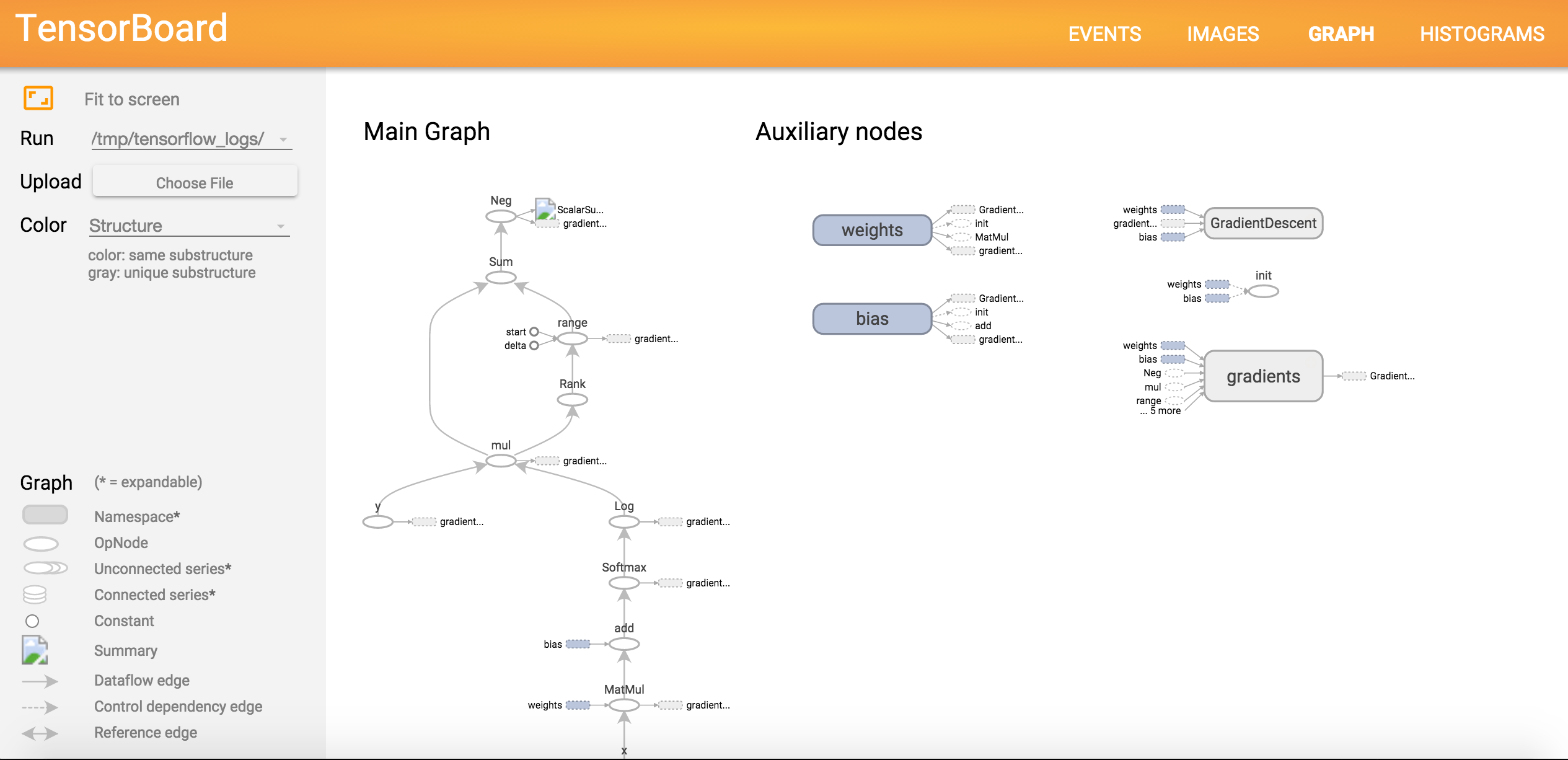
1.10 TensorFlow 图的可视化
致谢:派生于 Aymeric Damien 的 TensorFlow 示例
配置
参考配置指南。
import tensorflow as tfimport numpy# 导入 MINST 数据import input_datamnist = input_data.read_data_sets("/tmp/data/", one_hot=True)'''Extracting /tmp/data/train-images-idx3-ubyte.gzExtracting /tmp/data/train-labels-idx1-ubyte.gzExtracting /tmp/data/t10k-images-idx3-ubyte.gzExtracting /tmp/data/t10k-labels-idx1-ubyte.gz'''# 使用来自之前示例的 Logistic 回归# 参数learning_rate = 0.01training_epochs = 10batch_size = 100display_step = 1# TF 图输入x = tf.placeholder("float", [None, 784], name='x') # mnist 数据图像,形状为 28*28=784y = tf.placeholder("float", [None, 10], name='y') # 0-9 数字识别 => 10 个类# 创建模型# 设置模型权重W = tf.Variable(tf.zeros([784, 10]), name="weights")b = tf.Variable(tf.zeros([10]), name="bias")# 构造模型activation = tf.nn.softmax(tf.matmul(x, W) + b) # Softmax# 最小化交叉熵误差cost = -tf.reduce_sum(y*tf.log(activation)) # 交叉熵optimizer = tf.train.GradientDescentOptimizer(learning_rate).minimize(cost) # 梯度下降# 初始化变量init = tf.initialize_all_variables()# 加载图with tf.Session() as sess:sess.run(init)# 将日志写入器设为文件夹 '/tmp/tensorflow_logs'summary_writer = tf.train.SummaryWriter('/tmp/tensorflow_logs', graph_def=sess.graph_def)# 训练循环for epoch in range(training_epochs):avg_cost = 0.total_batch = int(mnist.train.num_examples/batch_size)# 遍历所有批量for i in range(total_batch):batch_xs, batch_ys = mnist.train.next_batch(batch_size)# 使用批量数据拟合训练sess.run(optimizer, feed_dict={x: batch_xs, y: batch_ys})# 计算平均损失avg_cost += sess.run(cost, feed_dict={x: batch_xs, y: batch_ys})/total_batch# 展示每一步的日志if epoch % display_step == 0:print "Epoch:", '%04d' % (epoch+1), "cost=", "{:.9f}".format(avg_cost)print "Optimization Finished!"# 测试模型correct_prediction = tf.equal(tf.argmax(activation, 1), tf.argmax(y, 1))# 计算准确率accuracy = tf.reduce_mean(tf.cast(correct_prediction, "float"))print "Accuracy:", accuracy.eval({x: mnist.test.images, y: mnist.test.labels})
运行命令行
tensorboard --logdir=/tmp/tensorflow_logs
在你的浏览器中打开 http://localhost:6006/
# 图的可视化# Tensorflow 使你很容易可视化所有计算图# 你可以点击图的任何部分,来获取更多细节
# 权重细节

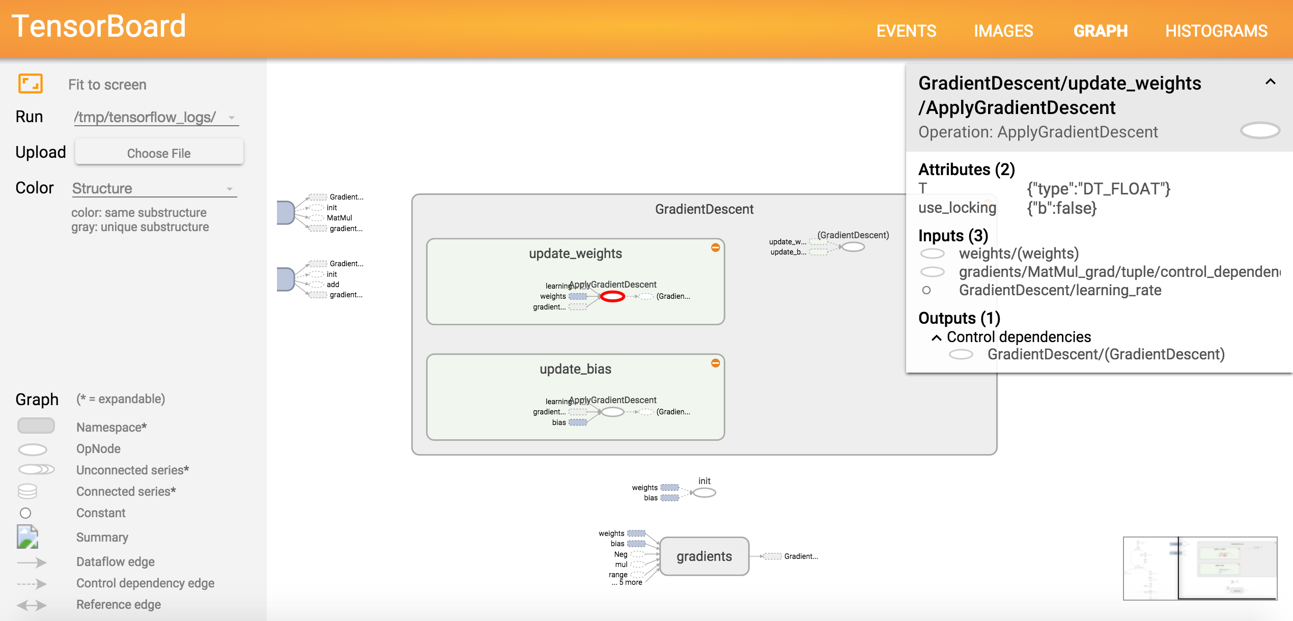
# 梯度下降细节
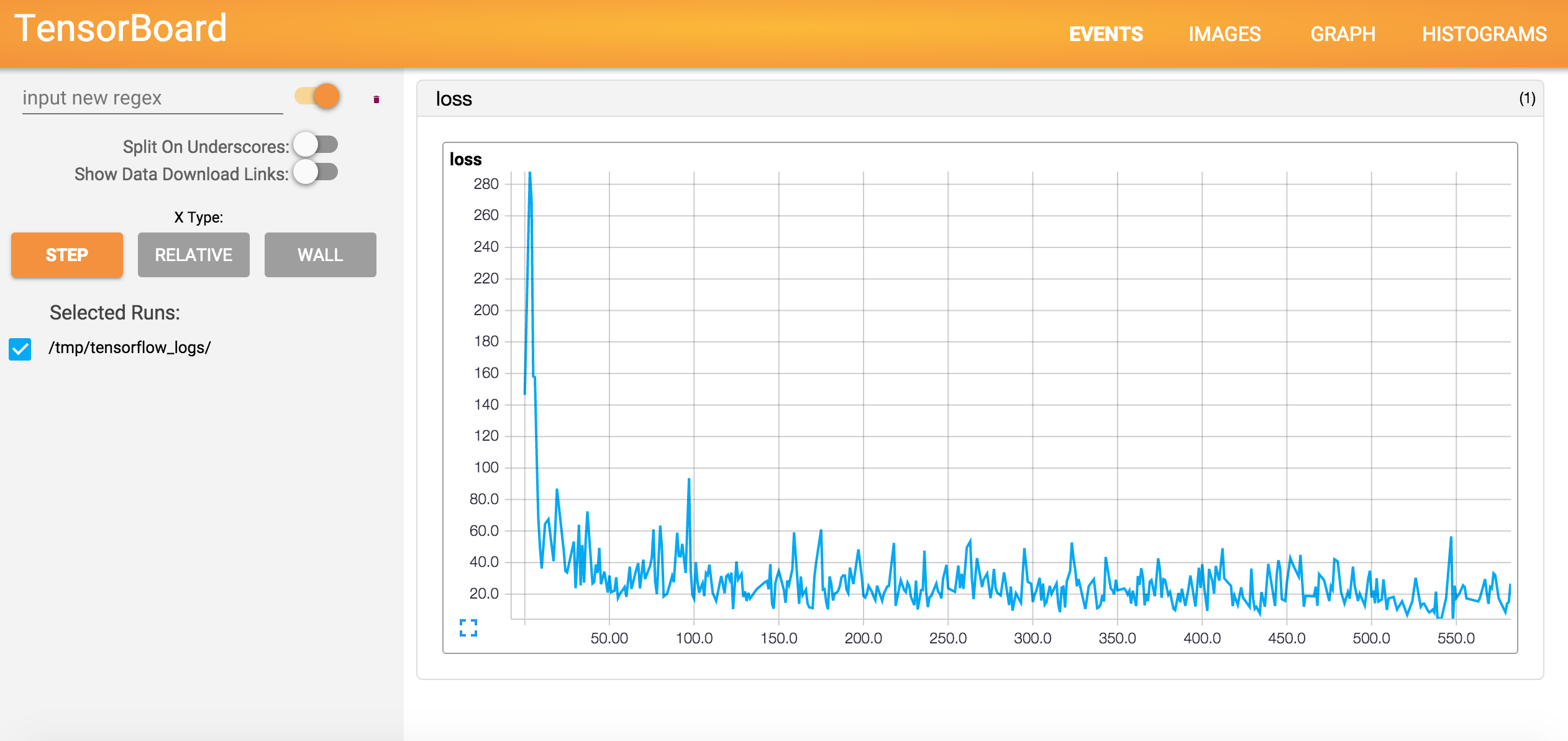
1.11 TensorFlow 损失可视化
致谢:派生于 Aymeric Damien 的 TensorFlow 示例
配置
参考配置指南。
import tensorflow as tfimport numpy# 导入 MINST 数据import input_datamnist = input_data.read_data_sets("/tmp/data/", one_hot=True)'''Extracting /tmp/data/train-images-idx3-ubyte.gzExtracting /tmp/data/train-labels-idx1-ubyte.gzExtracting /tmp/data/t10k-images-idx3-ubyte.gzExtracting /tmp/data/t10k-labels-idx1-ubyte.gz'''# 使用来自之前示例的 Logistic 回归# 参数learning_rate = 0.01training_epochs = 10batch_size = 100display_step = 1# TF 图输入x = tf.placeholder("float", [None, 784], name='x') # mnist 数据图像,形状为 28*28=784y = tf.placeholder("float", [None, 10], name='y') # 0-9 数字识别 => 10 个类# 创建模型# 设置模型权重W = tf.Variable(tf.zeros([784, 10]), name="weights")b = tf.Variable(tf.zeros([10]), name="bias")# 构造模型activation = tf.nn.softmax(tf.matmul(x, W) + b) # Softmax# 最小化交叉熵误差cost = -tf.reduce_sum(y*tf.log(activation)) # 交叉熵optimizer = tf.train.GradientDescentOptimizer(learning_rate).minimize(cost) # 梯度下降# 初始化变量init = tf.initialize_all_variables()# 创建汇总来监控损失函数tf.scalar_summary("loss", cost)# 将所有汇总合并为一个操作merged_summary_op = tf.merge_all_summaries()# 加载图with tf.Session() as sess:sess.run(init)# 将日志写入器设为文件夹 '/tmp/tensorflow_logs'summary_writer = tf.train.SummaryWriter('/tmp/tensorflow_logs', graph_def=sess.graph_def)# 训练循环for epoch in range(training_epochs):avg_cost = 0.total_batch = int(mnist.train.num_examples/batch_size)# 遍历所有批量for i in range(total_batch):batch_xs, batch_ys = mnist.train.next_batch(batch_size)# 使用批量数据拟合训练sess.run(optimizer, feed_dict={x: batch_xs, y: batch_ys})# 计算平均损失avg_cost += sess.run(cost, feed_dict={x: batch_xs, y: batch_ys})/total_batch# 在每个迭代中写日志summary_str = sess.run(merged_summary_op, feed_dict={x: batch_xs, y: batch_ys})summary_writer.add_summary(summary_str, epoch*total_batch + i)# 展示每一步的日志if epoch % display_step == 0:print "Epoch:", '%04d' % (epoch+1), "cost=", "{:.9f}".format(avg_cost)print "Optimization Finished!"# 测试模型correct_prediction = tf.equal(tf.argmax(activation, 1), tf.argmax(y, 1))# 计算准确率accuracy = tf.reduce_mean(tf.cast(correct_prediction, "float"))print "Accuracy:", accuracy.eval({x: mnist.test.images, y: mnist.test.labels})
运行命令行
tensorboard --logdir=/tmp/tensorflow_logs
在你的浏览器中打开 http://localhost:6006/
# 每个小批量步骤的损失

若有收获,就点个赞吧
0 人点赞
