chapter 1
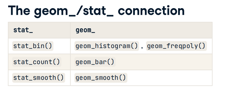
1.1 Stats with geoms
Two categories of functions:- Called from within a geom
- Called independently
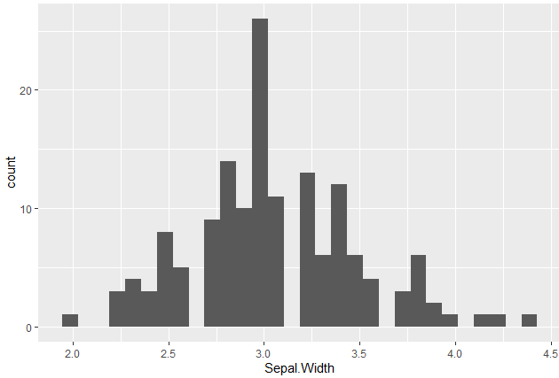
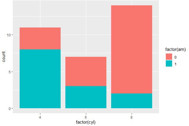
p <- ggplot(iris, aes(x = Sepal.Width))p + geom_histogram()p + stat_bin()p <- ggplot(mtcars, aes(x = factor(cyl), fill = factor(am)))p + geom_bar()p + stat_count()
 |
 |
|---|---|
ggplot(iris, aes(x = Sepal.Length, y = Sepal.Width, color = Species)) +geom_point() +geom_smooth()ggplot(iris, aes(x = Sepal.Length, y = Sepal.Width, color = Species)) +geom_point() +geom_smooth(se = FALSE, span = 0.4)ggplot(iris, aes(x = Sepal.Length, y = Sepal.Width, color = Species)) +geom_point() +geom_smooth(method = "lm", se = FALSE)ggplot(iris, aes(x = Sepal.Length, y = Sepal.Width, color = Species)) +geom_point() +geom_smooth(method = "lm", fullrange = TRUE)
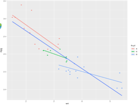
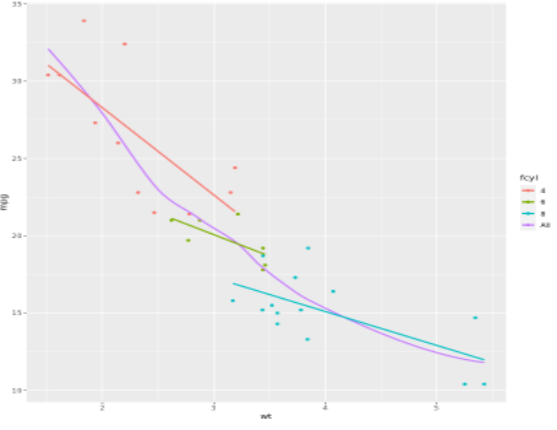
# Amend the plot to add another smooth layer with dummy groupingggplot(mtcars, aes(x = wt, y = mpg, color = fcyl)) +geom_point() +stat_smooth(method = "lm", se = FALSE) +stat_smooth(aes(group=1),method="lm",se=FALSE)# # Amend the plotggplot(mtcars, aes(x = wt, y = mpg, color = fcyl)) +geom_point() +# Map color to dummy variable "All"stat_smooth(aes(color="All"),se = FALSE) +stat_smooth(method = "lm", se = FALS
 |
 |
|---|---|
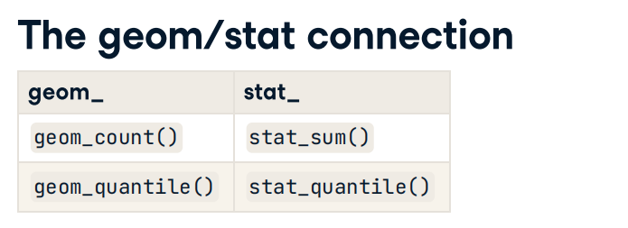
1.2 Stats: sum and quantile
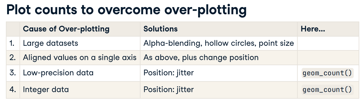
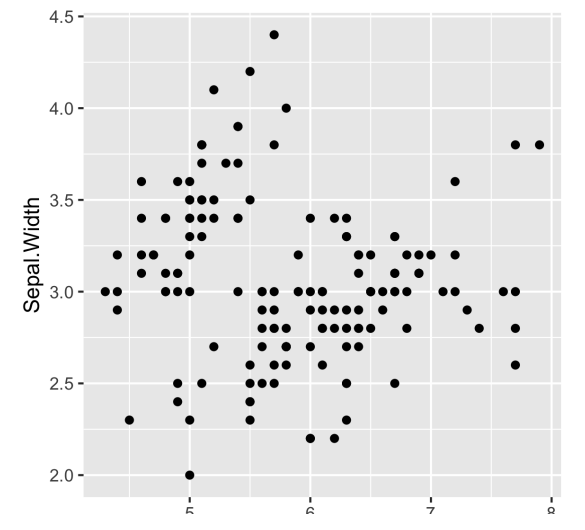
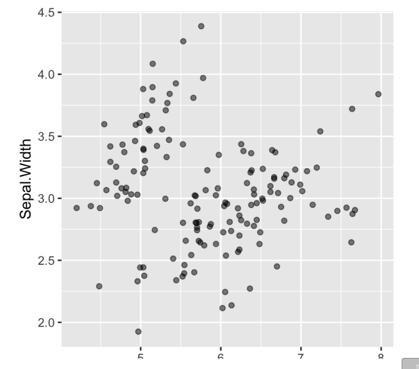
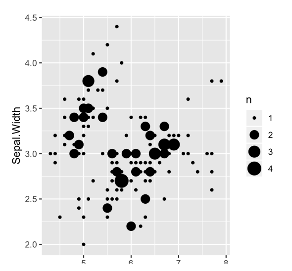
# Low precision (& integer) datap <- ggplot(iris, aes(Sepal.Length, Sepal.Width))p + geom_point()# Jittering may give a wrong impressionsp + geom_jitter(alpha = 0.5, width = 0.1, height = 0.1)p + geom_count()p + stat_sum()
 |
 |
 |
|---|---|---|
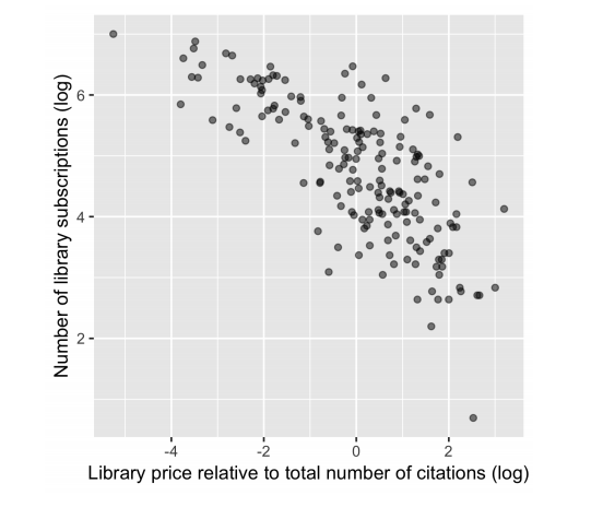
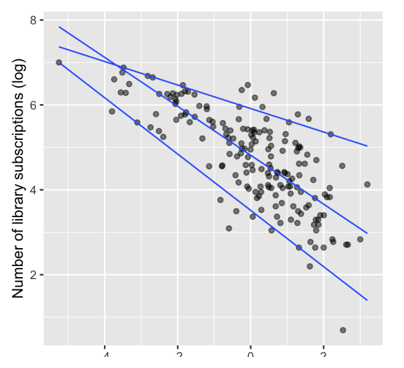
Linear regression predicts the mean response from the explanatory variables, quantile regression predicts a quantile response (e.g. the median) from the explanatory variables.
library(AER)data(Journals)p <- ggplot(Journals, aes(log(price/citations), log(subs))) +geom_point(alpha = 0.5)# Using geom_quantilesp + geom_quantile(quantiles = c(0.05, 0.50, 0.95))
 |
 |
|---|---|

若有收获,就点个赞吧
0 人点赞
