| 版本 | 日期 | 备注 |
|---|---|---|
| 1.0 | 2022.1.26 | 文章首发 |
0.前言
前阵子组里的小伙伴问我“为什么Flink从我们的代码到真正可执行的状态,要经过这么多个graph转换?这样做有什么好处嘛?”我早期看到这里的设计时的确有过相同的疑惑,当时由于手里还在看别的东西,查阅过一些资料后就翻页了。如今又碰到了这样的问题,不妨就在这篇文章中好好搞清楚。
本文的源码基于Flink
1.14.0。
1. 分层设计
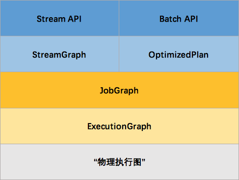
该图来自Jark大佬的博客:http://wuchong.me/blog/2016/05/03/flink-internals-overview/
以上是Flink的Graph层次图,在接下来的内容我们会逐一揭开它们的面纱,得知它们存在的意义。
1.1 BatchAPI的OptimizedPlan
在这个小节中,我们会看到DataSet从Plan转换到OptimizedPlan的过程中。为了方便读者有个概念,我们在这里解释一下几个名词:
- DataSet:面向用户的批处理API。
- Plan:描述DataSource以及DataSink以及Operation如何互动的计划。
- OptimizedPlan:优化过的执行计划。
代码入口:
|--ClientFrontend#main\-- parseAndRun\-- runApplication\-- getPackagedProgram\-- buildProgram\-- executeProgram|-- ClientUtils#executeProgram|-- PackagedProgram#invokeInteractiveModeForExecution\-- callMainMethod //调用用户编写的程序入口|-- ExecutionEnvironment#execute\-- executeAsync // 创建Plan|-- PipelineExecutorFactory#execute|-- EmbeddedExecutor#execute\-- submitAndGetJobClientFuture|-- PipelineExecutorUtils#getJobGraph|-- FlinkPipelineTranslationUtil#getJobGraph|-- FlinkPipelineTranslator#translateToJobGraph //如果传入的是Plan,则会在内部实现中先转换出OptimizedPlan,再转换到JobGraph;如果是StreamGraph,则会直接转换出JobGraph|-- PlanTranslator#translateToJobGraph\-- compilePlan
我们看一下这段代码:
private JobGraph compilePlan(Plan plan, Configuration optimizerConfiguration) {Optimizer optimizer = new Optimizer(new DataStatistics(), optimizerConfiguration);OptimizedPlan optimizedPlan = optimizer.compile(plan);JobGraphGenerator jobGraphGenerator = new JobGraphGenerator(optimizerConfiguration);return jobGraphGenerator.compileJobGraph(optimizedPlan, plan.getJobId());}
非常的清晰。就是从OptimizedPlan到JobGraph。OptimizedPlan的转换过程我们看Optimizer#compile方法。先看方法签名上的注释:
/*** Translates the given program to an OptimizedPlan. The optimized plan describes for each* operator which strategy to use (such as hash join versus sort-merge join), what data exchange* method to use (local pipe forward, shuffle, broadcast), what exchange mode to use (pipelined,* batch), where to cache intermediate results, etc,** <p>The optimization happens in multiple phases:** <ol>* <li>Create optimizer dag implementation of the program.* <p><tt>OptimizerNode</tt> representations of the PACTs, assign parallelism and compute* size estimates.* <li>Compute interesting properties and auxiliary structures.* <li>Enumerate plan alternatives. This cannot be done in the same step as the interesting* property computation (as opposed to the Database approaches), because we support plans* that are not trees.* </ol>** @param program The program to be translated.* @param postPasser The function to be used for post passing the optimizer's plan and setting* the data type specific serialization routines.* @return The optimized plan.* @throws CompilerException Thrown, if the plan is invalid or the optimizer encountered an* inconsistent situation during the compilation process.*/private OptimizedPlan compile(Plan program, OptimizerPostPass postPasser)
这里提到了会有好几步来做优化:
- 创建优化过的DAG,为其生成的OptimizerNode遵循PACT模型,并为其分配了并发度以及计算资源。
- 生成一些重要的属性以及辅助性数据结构。
- 枚举所有的代替方案。
在方法的实现中,会创建大量的Visitor来对程序做遍历优化。
1.1.1 GraphCreatingVisitor
首先是创建GraphCreatingVisitor,对原始的Plan进行优化,将每个operator优化成OptimizerNode,OptimizerNode之间通过DagConnection相连,DagConnection相当于一个边模型,有source和target,可以表示OptimizerNode的输入和输出。在这个过程中会做这些事:
- 为每个算子创建一个OptimizerNode——更加接近执行描述的Node(估算出数据的大小、data flow在哪里进行拆分和合并等)
- 用Channel将它们连接起来
- 根据建议生成相应的策略:Operator用什么策略执行:比如Hash Join or Sort Merge Join;Operator间的数据交换策略,是Local Pipe Forward、Shuffle,还是Broadcast;Operator间的数据交换模式,是Pipelined还是Batch。
1.1.2 IdAndEstimatesVisitor
顾名思义,为每个算子生成id,并估算其数据量。估算的实现见OptimizerNode#computeOutputEstimates——这是一个抽象函数,我们可以关注一下DataSourceNode里的实现,它会根据上游数据源的一系列属性(比如行数、大小)得出估算值。但这段代码放在这里并不合适
,作者的原意似乎是关注file类型的上游,注释这么说道:see, if we have a statistics object that can tell us a bit about the file。
1.1.3 UnionParallelismAndForwardEnforcer
这里会保证UnionNode的并发度与下游对其,避免数据分布有误而导致数据不精准(见https://github.com/apache/flink/pull/5742)。
1.1.4 BranchesVisitor
计算不会闭合的下游子DAG图。见其定义:
/*** Description of an unclosed branch. An unclosed branch is when the data flow branched (one* operator's result is consumed by multiple targets), but these different branches (targets)* have not been joined together.*/public static final class UnclosedBranchDescriptor {
1.1.5 InterestingPropertyVisitor
根据Node的属性估算成本。
估算算法见:node.computeInterestingPropertiesForInputs
- WorksetIterationNode
- TwoInputNode
- SingleInputNode
- BulkIterationNode
之后便会根据成本算出一系列的执行计划:
// the final step is now to generate the actual plan alternativesList<PlanNode> bestPlan = rootNode.getAlternativePlans(this.costEstimator);
在这里,OptimizerNode优化成了PlanNode,PlanNode是最终的优化节点类型,它包含了节点的更多属性,节点之间通过Channel进行连接,Channel也是一种边模型,同时确定了节点之间的数据交换方式ShipStrategyType和DataExchangeMode,ShipStrategyType表示的两个节点之间数据的传输策略,比如是否进行数据分区,进行hash分区,范围分区等; DataExchangeMode表示的是两个节点间数据交换的模式,有PIPELINED和BATCH,和ExecutionMode是一样的,ExecutionMode决定了DataExchangeMode——直接发下去还是先落盘。
1.1.6 PlanFinalizer.createFinalPlan
PlanFinalizer.createFinalPlan()。其大致的实现就是将节点添加到sources、sinks、allNodes中,还可能会为每个节点设置任务占用的内存等。
1.1.7 BinaryUnionReplacer
顾名思义,针对上游同样是Union的操作做去重替换,合并到一起。笔者认为,这在输出等价的情况下,减少了Node的生成。
1.1.8 RangePartitionRewriter
在使用范围分区这一特性时,需要尽可能保证各分区所处理的数据集均衡性以最大化利用计算资源并减少作业的执行时间。为此,优化器提供了范围分区重写器(RangePartitionRewriter)来对范围分区的分区策略进行优化,使其尽可能平均地分配数据,避免数据倾斜。
如果要尽可能的平均分配数据,肯定要对数据源进行估算。但显然是没法读取所有的数据进行估算的,这里Flink采用了ReservoirSampling算法的改良版——可以参考论文Optimal Random Sampling from Distributed Streams Revisited,在代码中由org.apache.flink.api.java.sampling.ReservoirSamplerWithReplacement和org.apache.flink.api.java.sampling.ReservoirSamplerWithoutReplacement实现。
值得一提的是,无论是
Plan还是OptimizerNode都实现了Visitable接口,这是典型的策略模式使用,这让代码变得非常灵活,正如注释所说的——遍历方式是可以自由编写的。
package org.apache.flink.util;import org.apache.flink.annotation.Internal;/*** This interface marks types as visitable during a traversal. The central method <i>accept(...)</i>* contains the logic about how to invoke the supplied {@link Visitor} on the visitable object, and* how to traverse further.** <p>This concept makes it easy to implement for example a depth-first traversal of a tree or DAG* with different types of logic during the traversal. The <i>accept(...)</i> method calls the* visitor and then send the visitor to its children (or predecessors). Using different types of* visitors, different operations can be performed during the traversal, while writing the actual* traversal code only once.** @see Visitor*/@Internalpublic interface Visitable<T extends Visitable<T>> {/*** Contains the logic to invoke the visitor and continue the traversal. Typically invokes the* pre-visit method of the visitor, then sends the visitor to the children (or predecessors) and* then invokes the post-visit method.** <p>A typical code example is the following:**<pre>{@code* public void accept(Visitor<Operator> visitor) {* boolean descend = visitor.preVisit(this);* if (descend) {* if (this.input != null) {* this.input.accept(visitor);* }* visitor.postVisit(this);* }* }* }</pre>** @param visitor The visitor to be called with this object as the parameter.* @see Visitor#preVisit(Visitable)* @see Visitor#postVisit(Visitable)*/void accept(Visitor<T> visitor);}
1.2 StreamAPI的StreamGraph
构造StreamGraph的入口函数是 StreamGraphGenerator.generate()。该函数会由触发程序执行的方法StreamExecutionEnvironment.execute()调用到。就像OptimizedPla,StreamGraph 也是在 Client 端构造的。
在这个过程中,流水线首先被转换为Transformation流水线,然后被映射为StreamGraph,该图与具体的执行无关,核心是表达计算过程的逻辑。
关于Transformation的引入,可以看社区的issue:https://issues.apache.org/jira/browse/FLINK-2398。本质是为了避免DataStream这一层对StreamGraph的耦合,因此引入这一层做解耦。
Transformation关注的属性偏向框架内部,如:name(算子名)、uid(job重启时分配之前相同的状态,持久保存状态)、bufferTimeout、parallelism、outputType、soltSharingGroup等。另外,Transformation分为物理Transformation和虚拟Transformation,这于下一层的StreamGraph实现是有关联的。
StreamGraph的核心对象有两个:
- StreamNode:它可以有多个输出,也可以有多个输入。由Transformation转换而来——实体的StreamNode会最终变成物算子,虚拟的StreamNode会附着在StreamEdge上。
- StreamEdge:StreamGraph的边,用于连接两个StreamNode。就像上面说的——一个StreamNode可以有多个出边、入边。StreamEdge中包含了旁路输出、分区器、字段筛选输出(与SQL Select中选择字段的逻辑一样)等的信息。
具体的转换代码在org.apache.flink.streaming.api.graph.StreamGraphGenerator中,每个Transformation都有对应的转换逻辑:
static {@SuppressWarnings("rawtypes")Map<Class<? extends Transformation>, TransformationTranslator<?, ? extends Transformation>>tmp = new HashMap<>();tmp.put(OneInputTransformation.class, new OneInputTransformationTranslator<>());tmp.put(TwoInputTransformation.class, new TwoInputTransformationTranslator<>());tmp.put(MultipleInputTransformation.class, new MultiInputTransformationTranslator<>());tmp.put(KeyedMultipleInputTransformation.class, new MultiInputTransformationTranslator<>());tmp.put(SourceTransformation.class, new SourceTransformationTranslator<>());tmp.put(SinkTransformation.class, new SinkTransformationTranslator<>());tmp.put(LegacySinkTransformation.class, new LegacySinkTransformationTranslator<>());tmp.put(LegacySourceTransformation.class, new LegacySourceTransformationTranslator<>());tmp.put(UnionTransformation.class, new UnionTransformationTranslator<>());tmp.put(PartitionTransformation.class, new PartitionTransformationTranslator<>());tmp.put(SideOutputTransformation.class, new SideOutputTransformationTranslator<>());tmp.put(ReduceTransformation.class, new ReduceTransformationTranslator<>());tmp.put(TimestampsAndWatermarksTransformation.class,new TimestampsAndWatermarksTransformationTranslator<>());tmp.put(BroadcastStateTransformation.class, new BroadcastStateTransformationTranslator<>());tmp.put(KeyedBroadcastStateTransformation.class,new KeyedBroadcastStateTransformationTranslator<>());translatorMap = Collections.unmodifiableMap(tmp);}
1.3 流批一体的JobGraph
代码入口和1.1小节几乎一摸一样,DataSet的入口类是ExecutionEnvironment,而DataStream的入口是StreamExecutionEnvironment。PlanTranslator变成了StreamGraphTranslator。所以,StreamGraph到JobGraph的转化也是在Client端进行的,主要工作做优化。其中非常重要的一个优化就是Operator Chain,它会将条件允许的算子合并到一起,避免跨线程、跨网络的传递。
是否开启OperationChain可以在程序中显示的调整。
接下来,我们来看下JobGraph到底是什么。先看注释:
/*** The JobGraph represents a Flink dataflow program, at the low level that the JobManager accepts.* All programs from higher level APIs are transformed into JobGraphs.** <p>The JobGraph is a graph of vertices and intermediate results that are connected together to* form a DAG. Note that iterations (feedback edges) are currently not encoded inside the JobGraph* but inside certain special vertices that establish the feedback channel amongst themselves.** <p>The JobGraph defines the job-wide configuration settings, while each vertex and intermediate* result define the characteristics of the concrete operation and intermediate data.*/public class JobGraph implements Serializable {
它是一张图,由vertices和intermediate组成。并且它是一个低等级的API,为JobMaster而生——所有高等级的API都会被转换成JobGraph。接下来我们需要关注的对象分别是JobVertex、JobEdge、IntermediateDataSet。其中,JobVertex的输入是JobEdge,输出是IntermediateDataSet。
1.3.1 JoBVertex
经过符合条件的多个StreamNode经过优化后的可能会融合在一起生成一个JobVertex,即一个JobVertex包含一个或多个算子(有兴趣的同学可以看StreamingJobGraphGenerator#buildChainedInputsAndGetHeadInputs或者阅读相关的Issue:https://issues.apache.org/jira/browse/FLINK-19434)。
1.3.2 JobEdge
JobEdge是连接IntermediateDatSet和JobVertex的边,代表着JobGraph中的一个数据流转通道,其上游是IntermediateDataSet,下游是JobVertex——数据通过JobEdge由IntermediateDataSet传递给目标JobVertex。
在这里,我们要关注它的一个成员变量:
/*** A distribution pattern determines, which sub tasks of a producing task are connected to which* consuming sub tasks.** <p>It affects how {@link ExecutionVertex} and {@link IntermediateResultPartition} are connected* in {@link EdgeManagerBuildUtil}*/public enum DistributionPattern {/** Each producing sub task is connected to each sub task of the consuming task. */ALL_TO_ALL,/** Each producing sub task is connected to one or more subtask(s) of the consuming task. */POINTWISE}
该分发模式会直接影响执行时Task之间的数据连接关系:点对点连接or全连接(或者叫广播)。
1.3.3 IntermediateDataSet
中间数据集IntermediateDataSet是一种逻辑结构,用来表示JobVertex的输出,即该JobVertex中包含的算子会产生的数据集。在这里我们需要关注ResultPartitionType:
- Blocking:顾名思义。都上游处理完数据后,再交给下游处理。这个数据分区可以被消费多次,也可以并发消费。这个分区并不会被自动销毁,而是交给调度器判断。
- BlokingPersistent:类似于Blocking,但是其生命周期由用户端指定。调用JobMaster或者ResourceManager的API来销毁,而不是由调度器控制。
- Pipelined:流交换模式。可以用于有界和无界流。这种分区类型的数据只能被每个消费者消费一次。且这种分区可以保留任意数据。
- PipelinedBounded:与Pipelined有些不同,这种分区保留的数据是有限的,这不会使数据和检查点延迟太久。因此适用于流计算场景(需注意,批处理模式下没有CheckpointBarrier)。
- Pipelined_Approximate:1.12引入的策略,用于针对单个task做fast failover的分区策略。有兴趣的同学可以阅读相关issue:https://issues.apache.org/jira/browse/FLINK-18112。
不同的执行模式下,其对应的结果分区类型不同,决定了在执行时刻数据交换的模式。
IntermediateDataSet的个数与该JobVertext对应的StreamNode的出边数量相同,可以是一个或者多个。
1.4 ExecutionGraph
JobManager接收到Client端提交的JobGraph及其依赖Jar之后就要开始调度运行该任务了,但JobGraph还是一个逻辑上的图,需要再进一步转化为并行化、可调度的执行图。这个动作是JobMaster做的——通过SchedulerBase触发,实际动作交给DefaultExecutionGraphBuilder#buildGraph来做。在这些动作中,会生成与JobVertex对应的ExecutionJobVertex(逻辑概念)和ExecutionVertex,与IntermediateDataSet对应的IntermediateResult(逻辑概念)和IntermediateResultPartition等,所谓的并行度也将通过上述类实现。
接下来要聊聊ExecutionGraph的一些细节,会涉及一些逻辑概念,因此在这里笔者画了一张图,便于参考。
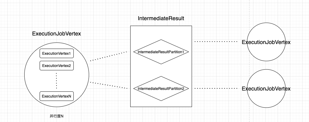
1.4.1 ExecutionJobVertex与ExecutionVertex
ExecutionJobVertex和JobGraph中的JobVertex一一对应。该对象还包含一组ExecutionVertex,数量与该JobVertex中所包含的StreamNode的并行度一致,如上图所示,如果并行度为N,那么就会有N个ExecutionVertex。所以每一个并行执行的实例就是ExecutionVertex。同时也会构建ExecutionVertex的输出IntermediateResult。
因此ExecutionJobVertex更像是一个逻辑概念。
1.4.2 IntermediaResult与IntermediaResultParitition
IntermediateResult表示ExecutionJobVertex的输出,和JobGraph中的IntermediateDataSet一一对应,该对象也是一个逻辑概念。同理,一个ExecutionJobVertex可以有多个中间结果,取决于当前JobVertex有几个出边(JobEdge)。
一个中间结果集包含多个中间结果分区IntermediateResultPartition,其个数等于该Job Vertext的并发度,或者叫作算子的并行度。每个IntermediateResultPartition表示1个ExecutionVertex输出结果。
1.4.3 Execution
ExecutionVertex在Runtime对应了一个Task。在真正执行的时会将ExecutionVerterx包装为一个Execution。
关于JobGraph如何提交到JobMaster不是本文的重点,有兴趣的同学可以自行查看
org.apache.flink.runtime.dispatcher.DispatcherGateway#submitJob的相关调用栈。
1.4.5 从JobGraph到ExecutionGraph
上面介绍了几个重要概念。接下来看一下ExecutionGraph的构建过程。主要参考方法为org.apache.flink.runtime.executiongraph.DefaultExecutionGraph#attachJobGraph。
首先是构建ExecutionJobVertex(参考其构造方法),设置其并行度、共享Solt、CoLocationGroup,并构建IntermediaResult与IntermediaResuktParitition,根据并发度创建ExecutionVertex,并检查IntermediateResults是否有重复引用。最后,会对可切分的数据源进行切分。
其次便是构建Edge(参考 org.apache.flink.runtime.executiongraph.EdgeManagerBuildUtil#connectVertexToResult)。根据DistributionPattern来创建EdgeManager,并将ExecutionVertex和IntermediateResult关联起来,为运行时建立Task之间的数据交换就是以此为基础建立数据的物理传输通道的。
1.4.6 开胃菜:从ExecutionGraph到真正的执行
当JobMaster生成ExecutionGraph后,便进入了作业调度阶段。这里面涉及到了不同的调度策略、资源申请、任务分发以及Failover的管理。涉及的内容极多,因此会在另外的文章中讨论。对此好奇的同学,可以先看DefaultExecutionGraphDeploymentTest#setupScheduler,里面的代码较为简单,可以观察ExecutionGraph到Scheduling的过程。
private SchedulerBase setupScheduler(JobVertex v1, int dop1, JobVertex v2, int dop2)throws Exception {v1.setParallelism(dop1);v2.setParallelism(dop2);v1.setInvokableClass(BatchTask.class);v2.setInvokableClass(BatchTask.class);DirectScheduledExecutorService executorService = new DirectScheduledExecutorService();// execution graph that executes actions synchronouslyfinal SchedulerBase scheduler =SchedulerTestingUtils.newSchedulerBuilder(JobGraphTestUtils.streamingJobGraph(v1, v2),ComponentMainThreadExecutorServiceAdapter.forMainThread()).setExecutionSlotAllocatorFactory(SchedulerTestingUtils.newSlotSharingExecutionSlotAllocatorFactory()).setFutureExecutor(executorService).setBlobWriter(blobWriter).build();final ExecutionGraph eg = scheduler.getExecutionGraph();checkJobOffloaded((DefaultExecutionGraph) eg);// schedule, this triggers mock deploymentscheduler.startScheduling();Map<ExecutionAttemptID, Execution> executions = eg.getRegisteredExecutions();assertEquals(dop1 + dop2, executions.size());return scheduler;}
2.小结
通过本文,我们了解各层图存在的意义:
- StreamGraph与OptimizedPlan:从外部API转向内部API,生成Graph的基本属性。如果是批处理,则会进行一系列的优化。
- JobGraph:流批统一的Graph。在这里做一些通用的优化,比如OperatorChain。
- ExecutionGraph:可执行级别的图,构建时关注大量的执行细节:如并发、Checkpoint配置有效性、监控打点设置、重复引用检查、可切分的数据源进行切分等等。
通过图的分层,Flink将不同的优化项、检查项放到了合适它们的层次,这也是单一职责原则的体现。

若有收获,就点个赞吧
0 人点赞
