1 简单回归问题
lesson3.pdf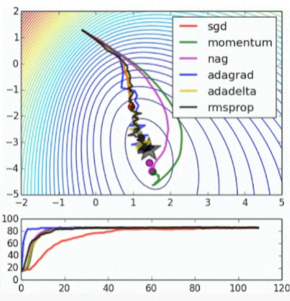
常用的也就sgd和rmsprop
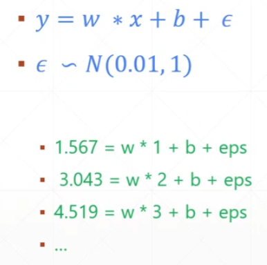
可以精确求解的方程组称为 Closed Form Solution
实际数据可能有噪声项
红色往低的蓝色走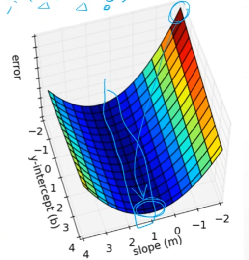
凸函数:Convex Optimization
2 回归问题实战
import numpy as npdef compute_error_for_line_given_points(b, w, points):""" 均方误差y = wx + b"""total_error, n = 0, len(points)for i in range(n):x, y = points[i] # 这批数据数据是一维的x,标记也是一维的ytotal_error += (y - (w * x + b)) ** 2return total_error / ndef step_gradient(b_current, w_current, points, learning_rate):b_gradient, w_gradient = 0, 0n = len(points)for i in range(n):x, y = points[i]# 损失函数关于b、w的梯度b_gradient += -(2 / n) * (y - ((w_current * x) + b_current))w_gradient += -(2 / n) * x * (y - ((w_current * x) + b_current))new_b = b_current - (learning_rate * b_gradient)new_m = w_current - (learning_rate * w_gradient)return new_b, new_mdef gradient_descent_runner(points, starting_b, starting_w, learning_rate, num_iterations):b, w = starting_b, starting_wfor i in range(num_iterations):b, w = step_gradient(b, w, np.array(points), learning_rate)return b, wdef run():points = np.genfromtxt("data.csv", delimiter=",")learning_rate = 0.0001initial_b = 0 # initial y-intercept guessinitial_m = 0 # initial slope guessnum_iterations = 1000print("Starting gradient descent at b = {0}, m = {1}, error = {2}".format(initial_b, initial_m,compute_error_for_line_given_points(initial_b, initial_m, points)))print("Running...")b, m = gradient_descent_runner(points, initial_b, initial_m, learning_rate, num_iterations)print("After {0} iterations b = {1}, m = {2}, error = {3}".format(num_iterations, b, m,compute_error_for_line_given_points(b, m, points)))if __name__ == '__main__':run()# 误差从5565降到112# Starting gradient descent at b = 0, m = 0, error = 5565.107834483211# Running...# After 1000 iterations b = 0.08893651993741346, m = 1.4777440851894448, error = 112.61481011613473
3 分类问题引入
one-hot编码方式(也叫独热编码,又称为一位有效编码)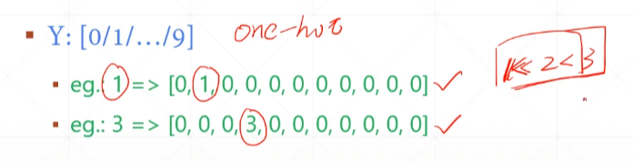
4 手写数字识别初体验
import torch
from torch import nn
from torch.nn import functional as F
from torch import optim

import torchvision
from matplotlib import pyplot as plt
____util = """
"""
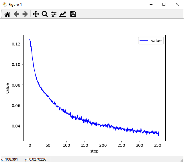
def plot_curve(data):
fig = plt.figure()
plt.plot(range(len(data)), data, color='blue')
plt.legend(['value'], loc='upper right')
plt.xlabel('step')
plt.ylabel('value')
plt.show()
def plot_image(img, label, name):
fig = plt.figure()
for i in range(6):
plt.subplot(2, 3, i + 1)
plt.tight_layout()
plt.imshow(img[i][0] * 0.3081 + 0.1307, cmap='gray', interpolation='none')
plt.title("{}: {}".format(name, label[i].item()))
plt.xticks([])
plt.yticks([])
plt.show()
def one_hot(label, depth=10):
out = torch.zeros(label.size(0), depth) # .size(0),获得第0维的大小
idx = torch.LongTensor(label).view(-1, 1)
out.scatter_(dim=1, index=idx, value=1)
return out
Load data
torch.utils.data.DataLoader
____mnist_train = """
"""
# step1. load dataset
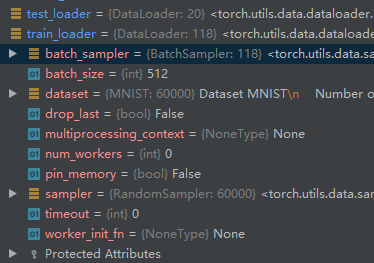
batch_size = 512
# 训练数据共6万张图(每张图28*28=784),每512张分为一个batch,共有118个batch
train_loader = torch.utils.data.DataLoader(
torchvision.datasets.MNIST('mnist_data', train=True, download=True,
transform=torchvision.transforms.Compose([ # 数据处理
torchvision.transforms.ToTensor(), # np转tensor
torchvision.transforms.Normalize( # 标准化
(0.1307,), (0.3081,))
])),
batch_size=batch_size, shuffle=True)
# 测试数据共1万张,分成20个batch
test_loader = torch.utils.data.DataLoader(
torchvision.datasets.MNIST('mnist_data/', train=False, download=True,
transform=torchvision.transforms.Compose([
torchvision.transforms.ToTensor(),
torchvision.transforms.Normalize(
(0.1307,), (0.3081,))
])),
batch_size=batch_size, shuffle=False)
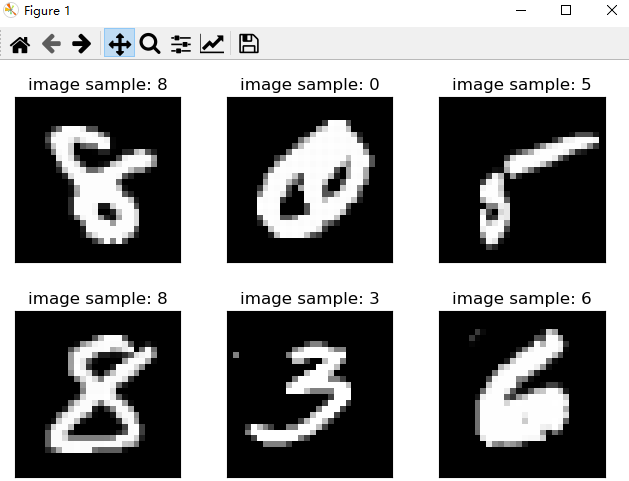
plot_image
def plot_image(img, label, name):
"""查看6张图效果"""
fig = plt.figure()
for i in range(6):
plt.subplot(2, 3, i + 1)
plt.tight_layout()
plt.imshow(img[i][0] * 0.3081 + 0.1307, cmap='gray', interpolation='none')
plt.title("{}: {}".format(name, label[i].item()))
plt.xticks([])
plt.yticks([])
plt.show()
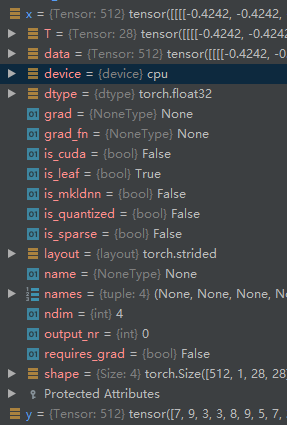
x, y = next(iter(train_loader)) # 获得一个batch的数据,x是数据特征,y是标记
print(x.shape, y.shape, x.min(), x.max())
# torch.Size([512, 1, 28, 28]) torch.Size([512]) tensor(-0.4242) tensor(2.8215)
# 如果去掉规范化,这里输出的最小最大值为:tensor(0.) tensor(1.)
plot_image(x, y, 'image sample')
Build Model
class Net(nn.Module):

    def __init__(self):
        super().__init__()

        # xw+b
        self.fc1 = nn.Linear(28 * 28, 256)
        self.fc2 = nn.Linear(256, 64)
        self.fc3 = nn.Linear(64, 10)

    def forward(self, x):
        # x: [b, 1, 28, 28]
        # h1 = relu(x*w1+b1)
        x = F.relu(self.fc1(x))
        # h2 = relu(h1*w2+b2)
        x = F.relu(self.fc2(x))
        # h3 = h2*w3+b3
        x = self.fc3(x)

        return x
Train
net = Net()
# [w1, b1, w2, b2, w3, b3]
optimizer = optim.SGD(net.parameters(), lr=0.01, momentum=0.9)

train_loss = []

for epoch in range(3):

    for batch_idx, (x, y) in enumerate(train_loader):

        # x: [b, 1, 28, 28], y: [512]
        # [b, 1, 28, 28] => [b, 784]
        x = x.view(x.size(0), 28 * 28)
        # => [b, 10]
        out = net(x)
        # [b, 10]
        y_onehot = one_hot(y)
        # loss = mse(out, y_onehot)
        loss = F.mse_loss(out, y_onehot)

        optimizer.zero_grad()  # 清零梯度
        loss.backward()
        # w' = w - lr*grad
        optimizer.step()

        train_loss.append(loss.item())

        if batch_idx % 10 == 0:
            print(epoch, batch_idx, loss.item())

plot_curve(train_loss)
# we get optimal [w1, b1, w2, b2, w3, b3]
Test
total_correct = 0
for x, y in test_loader:
x = x.view(x.size(0), 28 * 28)
out = net(x)
# out: [b, 10] => pred: [b]
pred = out.argmax(dim=1)
correct = pred.eq(y).sum().float().item()
total_correct += correct
total_num = len(test_loader.dataset)
acc = total_correct / total_num
print('test acc:', acc) # test acc: 0.8857
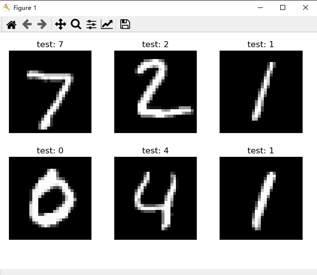
x, y = next(iter(test_loader))
out = net(x.view(x.size(0), 28 * 28))
pred = out.argmax(dim=1)
plot_image(x, pred, 'test')

若有收获,就点个赞吧
0 人点赞
