- Overview
- Linking with Spark
- Initializing Spark
- Resilient Distributed Datasets (RDDs)
- Shared Variables
- Deploying to a Cluster
- Launching Spark jobs from Java / Scala
- Unit Testing
-
Overview
At a high level, every Spark application consists of a driver program that runs the user’s
mainfunction and executes various parallel operations on a cluster. The main abstraction Spark provides is a resilient distributed dataset (RDD), which is a collection of elements partitioned across the nodes of the cluster that can be operated on in parallel. RDDs are created by starting with a file in the Hadoop file system (or any other Hadoop-supported file system), or an existing Scala collection in the driver program, and transforming it. Users may also ask Spark to persist an RDD in memory, allowing it to be reused efficiently across parallel operations. Finally, RDDs automatically recover from node failures.
A second abstraction in Spark is shared variables that can be used in parallel operations. By default, when Spark runs a function in parallel as a set of tasks on different nodes, it ships a copy of each variable used in the function to each task. Sometimes, a variable needs to be shared across tasks, or between tasks and the driver program. Spark supports two types of shared variables: broadcast variables, which can be used to cache a value in memory on all nodes, and accumulators, which are variables that are only “added” to, such as counters and sums.
This guide shows each of these features in each of Spark’s supported languages. It is easiest to follow along with if you launch Spark’s interactive shell – eitherbin/spark-shellfor the Scala shell orbin/pysparkfor the Python one.Linking with Spark
- Java
- Python
Spark 2.2.0 is built and distributed to work with Scala 2.11 by default. (Spark can be built to work with other versions of Scala, too.) To write applications in Scala, you will need to use a compatible Scala version (e.g. 2.11.X).
To write a Spark application, you need to add a Maven dependency on Spark. Spark is available through Maven Central at:
groupId = org.apache.sparkartifactId = spark-core_2.11version = 2.2.0
In addition, if you wish to access an HDFS cluster, you need to add a dependency on hadoop-client for your version of HDFS.
groupId = org.apache.hadoopartifactId = hadoop-clientversion = <your-hdfs-version>
Finally, you need to import some Spark classes into your program. Add the following lines:
import org.apache.spark.SparkContextimport org.apache.spark.SparkConf
(Before Spark 1.3.0, you need to explicitly import org.apache.spark.SparkContext._ to enable essential implicit conversions.)
Initializing Spark
The first thing a Spark program must do is to create a SparkContext object, which tells Spark how to access a cluster. To create a SparkContext you first need to build a SparkConf object that contains information about your application.
Only one SparkContext may be active per JVM. You must stop() the active SparkContext before creating a new one.
val conf = new SparkConf().setAppName(appName).setMaster(master)new SparkContext(conf)
The appName parameter is a name for your application to show on the cluster UI. master is a Spark, Mesos or YARN cluster URL, or a special “local” string to run in local mode. In practice, when running on a cluster, you will not want to hardcode master in the program, but rather launch the application with spark-submit and receive it there. However, for local testing and unit tests, you can pass “local” to run Spark in-process.
Using the Shell
In the Spark shell, a special interpreter-aware SparkContext is already created for you, in the variable called sc. Making your own SparkContext will not work. You can set which master the context connects to using the --master argument, and you can add JARs to the classpath by passing a comma-separated list to the --jars argument. You can also add dependencies (e.g. Spark Packages) to your shell session by supplying a comma-separated list of Maven coordinates to the --packages argument. Any additional repositories where dependencies might exist (e.g. Sonatype) can be passed to the --repositories argument. For example, to run bin/spark-shell on exactly four cores, use:
$ ./bin/spark-shell --master local[4]
Or, to also add code.jar to its classpath, use:
$ ./bin/spark-shell --master local[4] --jars code.jar
To include a dependency using Maven coordinates:
$ ./bin/spark-shell --master local[4] --packages "org.example:example:0.1"
For a complete list of options, run spark-shell --help. Behind the scenes, spark-shell invokes the more general spark-submit script.
Resilient Distributed Datasets (RDDs)
Spark revolves around the concept of a resilient distributed dataset (RDD), which is a fault-tolerant collection of elements that can be operated on in parallel. There are two ways to create RDDs: parallelizing an existing collection in your driver program, or referencing a dataset in an external storage system, such as a shared filesystem, HDFS, HBase, or any data source offering a Hadoop InputFormat.
Parallelized Collections
Parallelized collections are created by calling SparkContext’s parallelize method on an existing collection in your driver program (a Scala Seq). The elements of the collection are copied to form a distributed dataset that can be operated on in parallel. For example, here is how to create a parallelized collection holding the numbers 1 to 5:
val data = Array(1, 2, 3, 4, 5)val distData = sc.parallelize(data)
Once created, the distributed dataset (distData) can be operated on in parallel. For example, we might call distData.reduce((a, b) => a + b) to add up the elements of the array. We describe operations on distributed datasets later on.
One important parameter for parallel collections is the number of partitions to cut the dataset into. Spark will run one task for each partition of the cluster. Typically you want 2-4 partitions for each CPU in your cluster. Normally, Spark tries to set the number of partitions automatically based on your cluster. However, you can also set it manually by passing it as a second parameter to parallelize (e.g. sc.parallelize(data, 10)). Note: some places in the code use the term slices (a synonym for partitions) to maintain backward compatibility.
External Datasets
Spark can create distributed datasets from any storage source supported by Hadoop, including your local file system, HDFS, Cassandra, HBase, Amazon S3, etc. Spark supports text files, SequenceFiles, and any other Hadoop InputFormat.
Text file RDDs can be created using SparkContext’s textFile method. This method takes an URI for the file (either a local path on the machine, or a hdfs://, s3n://, etc URI) and reads it as a collection of lines. Here is an example invocation:
scala> val distFile = sc.textFile("data.txt")distFile: org.apache.spark.rdd.RDD[String] = data.txt MapPartitionsRDD[10] at textFile at <console>:26
Once created, distFile can be acted on by dataset operations. For example, we can add up the sizes of all the lines using the map and reduce operations as follows: distFile.map(s => s.length).reduce((a, b) => a + b).
Some notes on reading files with Spark:
- If using a path on the local filesystem, the file must also be accessible at the same path on worker nodes. Either copy the file to all workers or use a network-mounted shared file system.
- All of Spark’s file-based input methods, including
textFile, support running on directories, compressed files, and wildcards as well. For example, you can usetextFile("/my/directory"),textFile("/my/directory/*.txt"), andtextFile("/my/directory/*.gz"). - The
textFilemethod also takes an optional second argument for controlling the number of partitions of the file. By default, Spark creates one partition for each block of the file (blocks being 128MB by default in HDFS), but you can also ask for a higher number of partitions by passing a larger value. Note that you cannot have fewer partitions than blocks.
Apart from text files, Spark’s Scala API also supports several other data formats:
SparkContext.wholeTextFileslets you read a directory containing multiple small text files, and returns each of them as (filename, content) pairs. This is in contrast withtextFile, which would return one record per line in each file. Partitioning is determined by data locality which, in some cases, may result in too few partitions. For those cases,wholeTextFilesprovides an optional second argument for controlling the minimal number of partitions.- For SequenceFiles, use SparkContext’s
sequenceFile[K, V]method whereKandVare the types of key and values in the file. These should be subclasses of Hadoop’s Writable interface, like IntWritable and Text. In addition, Spark allows you to specify native types for a few common Writables; for example,sequenceFile[Int, String]will automatically read IntWritables and Texts. - For other Hadoop InputFormats, you can use the
SparkContext.hadoopRDDmethod, which takes an arbitraryJobConfand input format class, key class and value class. Set these the same way you would for a Hadoop job with your input source. You can also useSparkContext.newAPIHadoopRDDfor InputFormats based on the “new” MapReduce API (org.apache.hadoop.mapreduce). RDD.saveAsObjectFileandSparkContext.objectFilesupport saving an RDD in a simple format consisting of serialized Java objects. While this is not as efficient as specialized formats like Avro, it offers an easy way to save any RDD.
RDD Operations
RDDs support two types of operations: transformations, which create a new dataset from an existing one, and actions, which return a value to the driver program after running a computation on the dataset. For example,
mapis a transformation that passes each dataset element through a function and returns a new RDD representing the results. On the other hand,reduceis an action that aggregates all the elements of the RDD using some function and returns the final result to the driver program (although there is also a parallelreduceByKeythat returns a distributed dataset).
All transformations in Spark are lazy, in that they do not compute their results right away. Instead, they just remember the transformations applied to some base dataset (e.g. a file). The transformations are only computed when an action requires a result to be returned to the driver program. This design enables Spark to run more efficiently. For example, we can realize that a dataset created throughmapwill be used in areduceand return only the result of thereduceto the driver, rather than the larger mapped dataset.
By default, each transformed RDD may be recomputed each time you run an action on it. However, you may also persist an RDD in memory using thepersist(orcache) method, in which case Spark will keep the elements around on the cluster for much faster access the next time you query it. There is also support for persisting RDDs on disk, or replicated across multiple nodes.Basics
- Java
- Python
To illustrate RDD basics, consider the simple program below:
val lines = sc.textFile("data.txt")val lineLengths = lines.map(s => s.length)val totalLength = lineLengths.reduce((a, b) => a + b)
The first line defines a base RDD from an external file. This dataset is not loaded in memory or otherwise acted on: lines is merely a pointer to the file. The second line defines lineLengths as the result of a map transformation. Again, lineLengths is not immediately computed, due to laziness. Finally, we run reduce, which is an action. At this point Spark breaks the computation into tasks to run on separate machines, and each machine runs both its part of the map and a local reduction, returning only its answer to the driver program.
If we also wanted to use lineLengths again later, we could add:
lineLengths.persist()
before the reduce, which would cause lineLengths to be saved in memory after the first time it is computed.
Passing Functions to Spark
Spark’s API relies heavily on passing functions in the driver program to run on the cluster. There are two recommended ways to do this:
- Anonymous function syntax, which can be used for short pieces of code.
Static methods in a global singleton object. For example, you can define
object MyFunctionsand then passMyFunctions.func1, as follows:object MyFunctions {def func1(s: String): String = { ... }}myRdd.map(MyFunctions.func1)
Note that while it is also possible to pass a reference to a method in a class instance (as opposed to a singleton object), this requires sending the object that contains that class along with the method. For example, consider:
class MyClass {def func1(s: String): String = { ... }def doStuff(rdd: RDD[String]): RDD[String] = { rdd.map(func1) }}
Here, if we create a new
MyClassinstance and calldoStuffon it, themapinside there references thefunc1method of thatMyClassinstance, so the whole object needs to be sent to the cluster. It is similar to writingrdd.map(x => this.func1(x)).
In a similar way, accessing fields of the outer object will reference the whole object:class MyClass {val field = "Hello"def doStuff(rdd: RDD[String]): RDD[String] = { rdd.map(x => field + x) }}
is equivalent to writing
rdd.map(x => this.field + x), which references all ofthis. To avoid this issue, the simplest way is to copyfieldinto a local variable instead of accessing it externally:def doStuff(rdd: RDD[String]): RDD[String] = {val field_ = this.fieldrdd.map(x => field_ + x)}
Understanding closures
One of the harder things about Spark is understanding the scope and life cycle of variables and methods when executing code across a cluster. RDD operations that modify variables outside of their scope can be a frequent source of confusion. In the example below we’ll look at code that uses
foreach()to increment a counter, but similar issues can occur for other operations as well.Example
Consider the naive RDD element sum below, which may behave differently depending on whether execution is happening within the same JVM. A common example of this is when running Spark in
localmode (--master = local[n]) versus deploying a Spark application to a cluster (e.g. via spark-submit to YARN):- Java
-
var counter = 0var rdd = sc.parallelize(data)// Wrong: Don't do this!!rdd.foreach(x => counter += x)println("Counter value: " + counter)
Local vs. cluster modes
The behavior of the above code is undefined, and may not work as intended. To execute jobs, Spark breaks up the processing of RDD operations into tasks, each of which is executed by an executor. Prior to execution, Spark computes the task’s closure. The closure is those variables and methods which must be visible for the executor to perform its computations on the RDD (in this case
foreach()). This closure is serialized and sent to each executor.
The variables within the closure sent to each executor are now copies and thus, when counter is referenced within theforeachfunction, it’s no longer the counter on the driver node. There is still a counter in the memory of the driver node but this is no longer visible to the executors! The executors only see the copy from the serialized closure. Thus, the final value of counter will still be zero since all operations on counter were referencing the value within the serialized closure.
In local mode, in some circumstances theforeachfunction will actually execute within the same JVM as the driver and will reference the same original counter, and may actually update it.
To ensure well-defined behavior in these sorts of scenarios one should use anAccumulator. Accumulators in Spark are used specifically to provide a mechanism for safely updating a variable when execution is split up across worker nodes in a cluster. The Accumulators section of this guide discusses these in more detail.
In general, closures - constructs like loops or locally defined methods, should not be used to mutate some global state. Spark does not define or guarantee the behavior of mutations to objects referenced from outside of closures. Some code that does this may work in local mode, but that’s just by accident and such code will not behave as expected in distributed mode. Use an Accumulator instead if some global aggregation is needed.Printing elements of an RDD
Another common idiom is attempting to print out the elements of an RDD using
rdd.foreach(println)orrdd.map(println). On a single machine, this will generate the expected output and print all the RDD’s elements. However, inclustermode, the output tostdoutbeing called by the executors is now writing to the executor’sstdoutinstead, not the one on the driver, sostdouton the driver won’t show these! To print all elements on the driver, one can use thecollect()method to first bring the RDD to the driver node thus:rdd.collect().foreach(println). This can cause the driver to run out of memory, though, becausecollect()fetches the entire RDD to a single machine; if you only need to print a few elements of the RDD, a safer approach is to use thetake():rdd.take(100).foreach(println).Working with Key-Value Pairs
- Java
- Python
While most Spark operations work on RDDs containing any type of objects, a few special operations are only available on RDDs of key-value pairs. The most common ones are distributed “shuffle” operations, such as grouping or aggregating the elements by a key.
In Scala, these operations are automatically available on RDDs containing Tuple2 objects (the built-in tuples in the language, created by simply writing (a, b)). The key-value pair operations are available in the PairRDDFunctions class, which automatically wraps around an RDD of tuples.
For example, the following code uses the reduceByKey operation on key-value pairs to count how many times each line of text occurs in a file:
val lines = sc.textFile("data.txt")val pairs = lines.map(s => (s, 1))val counts = pairs.reduceByKey((a, b) => a + b)
We could also use counts.sortByKey(), for example, to sort the pairs alphabetically, and finally counts.collect() to bring them back to the driver program as an array of objects.
Note: when using custom objects as the key in key-value pair operations, you must be sure that a custom equals() method is accompanied with a matching hashCode() method. For full details, see the contract outlined in the Object.hashCode() documentation).
Transformations
The following table lists some of the common transformations supported by Spark. Refer to the RDD API doc (Scala, Java, Python, R) and pair RDD functions doc (Scala, Java) for details.
| Transformation | Meaning |
|---|---|
| map(func) | Return a new distributed dataset formed by passing each element of the source through a function func. |
| filter(func) | Return a new dataset formed by selecting those elements of the source on which func returns true. |
| flatMap(func) | Similar to map, but each input item can be mapped to 0 or more output items (so func should return a Seq rather than a single item). |
| mapPartitions(func) | Similar to map, but runs separately on each partition (block) of the RDD, so func must be of type Iterator |
| mapPartitionsWithIndex(func) | Similar to mapPartitions, but also provides func with an integer value representing the index of the partition, so func must be of type (Int, Iterator |
| sample(withReplacement, fraction, seed) | Sample a fraction fraction of the data, with or without replacement, using a given random number generator seed. |
| union(otherDataset) | Return a new dataset that contains the union of the elements in the source dataset and the argument. |
| intersection(otherDataset) | Return a new RDD that contains the intersection of elements in the source dataset and the argument. |
| distinct([numTasks])) | Return a new dataset that contains the distinct elements of the source dataset. |
| groupByKey([numTasks]) | When called on a dataset of (K, V) pairs, returns a dataset of (K, Iterable Note: If you are grouping in order to perform an aggregation (such as a sum or average) over each key, using reduceByKey or aggregateByKey will yield much better performance.Note: By default, the level of parallelism in the output depends on the number of partitions of the parent RDD. You can pass an optional numTasks argument to set a different number of tasks. |
| reduceByKey(func, [numTasks]) | When called on a dataset of (K, V) pairs, returns a dataset of (K, V) pairs where the values for each key are aggregated using the given reduce function func, which must be of type (V,V) => V. Like in groupByKey, the number of reduce tasks is configurable through an optional second argument. |
| aggregateByKey(zeroValue)(seqOp, combOp, [numTasks]) | When called on a dataset of (K, V) pairs, returns a dataset of (K, U) pairs where the values for each key are aggregated using the given combine functions and a neutral “zero” value. Allows an aggregated value type that is different than the input value type, while avoiding unnecessary allocations. Like in groupByKey, the number of reduce tasks is configurable through an optional second argument. |
| sortByKey([ascending], [numTasks]) | When called on a dataset of (K, V) pairs where K implements Ordered, returns a dataset of (K, V) pairs sorted by keys in ascending or descending order, as specified in the boolean ascending argument. |
| join(otherDataset, [numTasks]) | When called on datasets of type (K, V) and (K, W), returns a dataset of (K, (V, W)) pairs with all pairs of elements for each key. Outer joins are supported through leftOuterJoin, rightOuterJoin, and fullOuterJoin. |
| cogroup(otherDataset, [numTasks]) | When called on datasets of type (K, V) and (K, W), returns a dataset of (K, (IterablegroupWith. |
| cartesian(otherDataset) | When called on datasets of types T and U, returns a dataset of (T, U) pairs (all pairs of elements). |
| pipe(command, [envVars]) | Pipe each partition of the RDD through a shell command, e.g. a Perl or bash script. RDD elements are written to the process’s stdin and lines output to its stdout are returned as an RDD of strings. |
| coalesce(numPartitions) | Decrease the number of partitions in the RDD to numPartitions. Useful for running operations more efficiently after filtering down a large dataset. |
| repartition(numPartitions) | Reshuffle the data in the RDD randomly to create either more or fewer partitions and balance it across them. This always shuffles all data over the network. |
| repartitionAndSortWithinPartitions(partitioner) | Repartition the RDD according to the given partitioner and, within each resulting partition, sort records by their keys. This is more efficient than calling repartition and then sorting within each partition because it can push the sorting down into the shuffle machinery. |
Actions
The following table lists some of the common actions supported by Spark. Refer to the RDD API doc (Scala, Java, Python, R)
and pair RDD functions doc (Scala, Java) for details.
| Action | Meaning |
|---|---|
| reduce(func) | Aggregate the elements of the dataset using a function func (which takes two arguments and returns one). The function should be commutative and associative so that it can be computed correctly in parallel. |
| collect() | Return all the elements of the dataset as an array at the driver program. This is usually useful after a filter or other operation that returns a sufficiently small subset of the data. |
| count() | Return the number of elements in the dataset. |
| first() | Return the first element of the dataset (similar to take(1)). |
| take(n) | Return an array with the first n elements of the dataset. |
| takeSample(withReplacement, num, [seed]) | Return an array with a random sample of num elements of the dataset, with or without replacement, optionally pre-specifying a random number generator seed. |
| takeOrdered(n, [ordering]) | Return the first n elements of the RDD using either their natural order or a custom comparator. |
| saveAsTextFile(path) | Write the elements of the dataset as a text file (or set of text files) in a given directory in the local filesystem, HDFS or any other Hadoop-supported file system. Spark will call toString on each element to convert it to a line of text in the file. |
| saveAsSequenceFile(path) (Java and Scala) |
Write the elements of the dataset as a Hadoop SequenceFile in a given path in the local filesystem, HDFS or any other Hadoop-supported file system. This is available on RDDs of key-value pairs that implement Hadoop’s Writable interface. In Scala, it is also available on types that are implicitly convertible to Writable (Spark includes conversions for basic types like Int, Double, String, etc). |
| saveAsObjectFile(path) (Java and Scala) |
Write the elements of the dataset in a simple format using Java serialization, which can then be loaded using SparkContext.objectFile(). |
| countByKey() | Only available on RDDs of type (K, V). Returns a hashmap of (K, Int) pairs with the count of each key. |
| foreach(func) | Run a function func on each element of the dataset. This is usually done for side effects such as updating an Accumulator or interacting with external storage systems. Note: modifying variables other than Accumulators outside of the foreach() may result in undefined behavior. See Understanding closures for more details. |
The Spark RDD API also exposes asynchronous versions of some actions, like foreachAsync for foreach, which immediately return a FutureAction to the caller instead of blocking on completion of the action. This can be used to manage or wait for the asynchronous execution of the action.
Shuffle operations
Certain operations within Spark trigger an event known as the shuffle. The shuffle is Spark’s mechanism for re-distributing data so that it’s grouped differently across partitions. This typically involves copying data across executors and machines, making the shuffle a complex and costly operation.
Background
To understand what happens during the shuffle we can consider the example of the reduceByKey operation. The reduceByKey operation generates a new RDD where all values for a single key are combined into a tuple - the key and the result of executing a reduce function against all values associated with that key. The challenge is that not all values for a single key necessarily reside on the same partition, or even the same machine, but they must be co-located to compute the result.
In Spark, data is generally not distributed across partitions to be in the necessary place for a specific operation. During computations, a single task will operate on a single partition - thus, to organize all the data for a single reduceByKey reduce task to execute, Spark needs to perform an all-to-all operation. It must read from all partitions to find all the values for all keys, and then bring together values across partitions to compute the final result for each key - this is called the shuffle.
Although the set of elements in each partition of newly shuffled data will be deterministic, and so is the ordering of partitions themselves, the ordering of these elements is not. If one desires predictably ordered data following shuffle then it’s possible to use:
mapPartitionsto sort each partition using, for example,.sortedrepartitionAndSortWithinPartitionsto efficiently sort partitions while simultaneously repartitioningsortByto make a globally ordered RDD
Operations which can cause a shuffle include repartition operations like repartition and coalesce, ‘ByKey operations (except for counting) like groupByKey and reduceByKey, and join operations like cogroup and join.
Performance Impact
The Shuffle is an expensive operation since it involves disk I/O, data serialization, and network I/O. To organize data for the shuffle, Spark generates sets of tasks - map tasks to organize the data, and a set of reduce tasks to aggregate it. This nomenclature comes from MapReduce and does not directly relate to Spark’s map and reduce operations.
Internally, results from individual map tasks are kept in memory until they can’t fit. Then, these are sorted based on the target partition and written to a single file. On the reduce side, tasks read the relevant sorted blocks.
Certain shuffle operations can consume significant amounts of heap memory since they employ in-memory data structures to organize records before or after transferring them. Specifically, reduceByKey and aggregateByKey create these structures on the map side, and 'ByKey operations generate these on the reduce side. When data does not fit in memory Spark will spill these tables to disk, incurring the additional overhead of disk I/O and increased garbage collection.
Shuffle also generates a large number of intermediate files on disk. As of Spark 1.3, these files are preserved until the corresponding RDDs are no longer used and are garbage collected. This is done so the shuffle files don’t need to be re-created if the lineage is re-computed. Garbage collection may happen only after a long period of time, if the application retains references to these RDDs or if GC does not kick in frequently. This means that long-running Spark jobs may consume a large amount of disk space. The temporary storage directory is specified by the spark.local.dir configuration parameter when configuring the Spark context.
Shuffle behavior can be tuned by adjusting a variety of configuration parameters. See the ‘Shuffle Behavior’ section within the Spark Configuration Guide.
RDD Persistence
One of the most important capabilities in Spark is persisting (or caching) a dataset in memory across operations. When you persist an RDD, each node stores any partitions of it that it computes in memory and reuses them in other actions on that dataset (or datasets derived from it). This allows future actions to be much faster (often by more than 10x). Caching is a key tool for iterative algorithms and fast interactive use.
You can mark an RDD to be persisted using the persist() or cache() methods on it. The first time it is computed in an action, it will be kept in memory on the nodes. Spark’s cache is fault-tolerant – if any partition of an RDD is lost, it will automatically be recomputed using the transformations that originally created it.
In addition, each persisted RDD can be stored using a different storage level, allowing you, for example, to persist the dataset on disk, persist it in memory but as serialized Java objects (to save space), replicate it across nodes. These levels are set by passing a StorageLevel object (Scala, Java, Python) to persist(). The cache() method is a shorthand for using the default storage level, which is StorageLevel.MEMORY_ONLY (store deserialized objects in memory). The full set of storage levels is:
| Storage Level | Meaning |
|---|---|
| MEMORY_ONLY | Store RDD as deserialized Java objects in the JVM. If the RDD does not fit in memory, some partitions will not be cached and will be recomputed on the fly each time they’re needed. This is the default level. |
| MEMORY_AND_DISK | Store RDD as deserialized Java objects in the JVM. If the RDD does not fit in memory, store the partitions that don’t fit on disk, and read them from there when they’re needed. |
| MEMORY_ONLY_SER (Java and Scala) |
Store RDD as serialized Java objects (one byte array per partition). This is generally more space-efficient than deserialized objects, especially when using a fast serializer, but more CPU-intensive to read. |
| MEMORY_AND_DISK_SER (Java and Scala) |
Similar to MEMORY_ONLY_SER, but spill partitions that don’t fit in memory to disk instead of recomputing them on the fly each time they’re needed. |
| DISK_ONLY | Store the RDD partitions only on disk. |
| MEMORY_ONLY_2, MEMORY_AND_DISK_2, etc. | Same as the levels above, but replicate each partition on two cluster nodes. |
| OFF_HEAP (experimental) | Similar to MEMORY_ONLY_SER, but store the data in off-heap memory. This requires off-heap memory to be enabled. |
Note: In Python, stored objects will always be serialized with the Pickle library, so it does not matter whether you choose a serialized level. The available storage levels in Python include MEMORY_ONLY, MEMORY_ONLY_2, MEMORY_AND_DISK, MEMORY_AND_DISK_2, DISK_ONLY, and DISK_ONLY_2.
Spark also automatically persists some intermediate data in shuffle operations (e.g. reduceByKey), even without users calling persist. This is done to avoid recomputing the entire input if a node fails during the shuffle. We still recommend users call persist on the resulting RDD if they plan to reuse it.
Which Storage Level to Choose?
Spark’s storage levels are meant to provide different trade-offs between memory usage and CPU efficiency. We recommend going through the following process to select one:
- If your RDDs fit comfortably with the default storage level (
MEMORY_ONLY), leave them that way. This is the most CPU-efficient option, allowing operations on the RDDs to run as fast as possible. - If not, try using
MEMORY_ONLY_SERand selecting a fast serialization library to make the objects much more space-efficient, but still reasonably fast to access. (Java and Scala) - Don’t spill to disk unless the functions that computed your datasets are expensive, or they filter a large amount of the data. Otherwise, recomputing a partition may be as fast as reading it from disk.
Use the replicated storage levels if you want fast fault recovery (e.g. if using Spark to serve requests from a web application). All the storage levels provide full fault tolerance by recomputing lost data, but the replicated ones let you continue running tasks on the RDD without waiting to recompute a lost partition.
Removing Data
Spark automatically monitors cache usage on each node and drops out old data partitions in a least-recently-used (LRU) fashion. If you would like to manually remove an RDD instead of waiting for it to fall out of the cache, use the
RDD.unpersist()method.Shared Variables
Normally, when a function passed to a Spark operation (such as
maporreduce) is executed on a remote cluster node, it works on separate copies of all the variables used in the function. These variables are copied to each machine, and no updates to the variables on the remote machine are propagated back to the driver program. Supporting general, read-write shared variables across tasks would be inefficient. However, Spark does provide two limited types of shared variables for two common usage patterns: broadcast variables and accumulators.Broadcast Variables
Broadcast variables allow the programmer to keep a read-only variable cached on each machine rather than shipping a copy of it with tasks. They can be used, for example, to give every node a copy of a large input dataset in an efficient manner. Spark also attempts to distribute broadcast variables using efficient broadcast algorithms to reduce communication cost.
Spark actions are executed through a set of stages, separated by distributed “shuffle” operations. Spark automatically broadcasts the common data needed by tasks within each stage. The data broadcasted this way is cached in serialized form and deserialized before running each task. This means that explicitly creating broadcast variables is only useful when tasks across multiple stages need the same data or when caching the data in deserialized form is important.
Broadcast variables are created from a variablevby callingSparkContext.broadcast(v). The broadcast variable is a wrapper aroundv, and its value can be accessed by calling thevaluemethod. The code below shows this:- Java
-
scala> val broadcastVar = sc.broadcast(Array(1, 2, 3))broadcastVar: org.apache.spark.broadcast.Broadcast[Array[Int]] = Broadcast(0)scala> broadcastVar.valueres0: Array[Int] = Array(1, 2, 3)
After the broadcast variable is created, it should be used instead of the value
vin any functions run on the cluster so thatvis not shipped to the nodes more than once. In addition, the objectvshould not be modified after it is broadcast in order to ensure that all nodes get the same value of the broadcast variable (e.g. if the variable is shipped to a new node later).Accumulators
Accumulators are variables that are only “added” to through an associative and commutative operation and can therefore be efficiently supported in parallel. They can be used to implement counters (as in MapReduce) or sums. Spark natively supports accumulators of numeric types, and programmers can add support for new types.
As a user, you can create named or unnamed accumulators. As seen in the image below, a named accumulator (in this instancecounter) will display in the web UI for the stage that modifies that accumulator. Spark displays the value for each accumulator modified by a task in the “Tasks” table.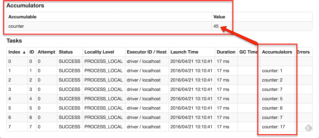
Tracking accumulators in the UI can be useful for understanding the progress of running stages (NOTE: this is not yet supported in Python). - Java
- Python
A numeric accumulator can be created by calling SparkContext.longAccumulator() or SparkContext.doubleAccumulator() to accumulate values of type Long or Double, respectively. Tasks running on a cluster can then add to it using the add method. However, they cannot read its value. Only the driver program can read the accumulator’s value, using its value method.
The code below shows an accumulator being used to add up the elements of an array:
scala> val accum = sc.longAccumulator("My Accumulator")accum: org.apache.spark.util.LongAccumulator = LongAccumulator(id: 0, name: Some(My Accumulator), value: 0)scala> sc.parallelize(Array(1, 2, 3, 4)).foreach(x => accum.add(x))...10/09/29 18:41:08 INFO SparkContext: Tasks finished in 0.317106 sscala> accum.valueres2: Long = 10
While this code used the built-in support for accumulators of type Long, programmers can also create their own types by subclassing AccumulatorV2. The AccumulatorV2 abstract class has several methods which one has to override: reset for resetting the accumulator to zero, add for adding another value into the accumulator, merge for merging another same-type accumulator into this one. Other methods that must be overridden are contained in the API documentation. For example, supposing we had a MyVector class representing mathematical vectors, we could write:
class VectorAccumulatorV2 extends AccumulatorV2[MyVector, MyVector] {private val myVector: MyVector = MyVector.createZeroVectordef reset(): Unit = {myVector.reset()}def add(v: MyVector): Unit = {myVector.add(v)}...}// Then, create an Accumulator of this type:val myVectorAcc = new VectorAccumulatorV2// Then, register it into spark context:sc.register(myVectorAcc, "MyVectorAcc1")
Note that, when programmers define their own type of AccumulatorV2, the resulting type can be different than that of the elements added.
For accumulator updates performed inside actions only, Spark guarantees that each task’s update to the accumulator will only be applied once, i.e. restarted tasks will not update the value. In transformations, users should be aware of that each task’s update may be applied more than once if tasks or job stages are re-executed.
Accumulators do not change the lazy evaluation model of Spark. If they are being updated within an operation on an RDD, their value is only updated once that RDD is computed as part of an action. Consequently, accumulator updates are not guaranteed to be executed when made within a lazy transformation like map(). The below code fragment demonstrates this property:
- Scala
- Java
- Python
val accum = sc.longAccumulatordata.map { x => accum.add(x); x }// Here, accum is still 0 because no actions have caused the map operation to be computed.
Deploying to a Cluster
The application submission guide describes how to submit applications to a cluster. In short, once you package your application into a JAR (for Java/Scala) or a set of.pyor.zipfiles (for Python), thebin/spark-submitscript lets you submit it to any supported cluster manager.Launching Spark jobs from Java / Scala
The org.apache.spark.launcher package provides classes for launching Spark jobs as child processes using a simple Java API.Unit Testing
Spark is friendly to unit testing with any popular unit test framework. Simply create aSparkContextin your test with the master URL set tolocal, run your operations, and then callSparkContext.stop()to tear it down. Make sure you stop the context within afinallyblock or the test framework’stearDownmethod, as Spark does not support two contexts running concurrently in the same program.Where to Go from Here
You can see some example Spark programs on the Spark website. In addition, Spark includes several samples in theexamplesdirectory (Scala, Java, Python, R). You can run Java and Scala examples by passing the class name to Spark’sbin/run-examplescript; for instance:
For Python examples, use./bin/run-example SparkPi
spark-submitinstead:
For R examples, use./bin/spark-submit examples/src/main/python/pi.py
spark-submitinstead:
For help on optimizing your programs, the configuration and tuning guides provide information on best practices. They are especially important for making sure that your data is stored in memory in an efficient format. For help on deploying, the cluster mode overview describes the components involved in distributed operation and supported cluster managers../bin/spark-submit examples/src/main/r/dataframe.R
Finally, full API documentation is available in Scala, Java, Python and R.

若有收获,就点个赞吧
0 人点赞
