1.前言
算法原理可以参考:https://zhuanlan.zhihu.com/p/102984842
Non_Local_Block是受图像去噪算法Non_Local_Mean的启发,而被发明的,使得卷积神经网络不仅仅是关注局部的信息,也通过Non Local Block使得feature map也更加关注全局的信息。
Non Local Mean算法的讲解可以参考我的这一篇博客:https://www.yuque.com/u487847/alpre9/cfiana
同时Non Local Mean不仅仅被正式是CV中attention的一种范式之一,而且在对抗学习中也有着应用,为了减少对抗学习中一些噪声对特征图的干扰(feature noise),提出了通过Non Local Block进行feature denoising,实验证明该方法对feature map噪声起到了抑制的作用。
具体文章可以参考:https://blog.csdn.net/weixin_43578873/article/details/105192189
2.算法的原理简述


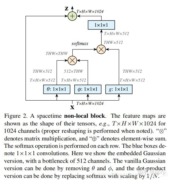
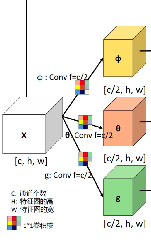
X是一个feature map,形状为[bs, c, h, w], 经过三个1×1卷积核,将通道缩减为原来一半(c/2)。
然后将h,w两个维度进行flatten,变为h×w,最终形状为[bs, c/2, h×w]的tensor。
对θ对应的tensor进行通道重排,在线性代数中也就是转置,得到形状为[bs, h×w, c/2]。
然后与φ代表的tensor进行矩阵乘法,得到一个形状为[bs, h×w,h×w]的矩阵,这个矩阵计算的是相似度(或者理解为attention)。
然后经过softmax进行归一化,然后将该得到的矩阵 与g 经过flatten和转置的结果进行矩阵相乘,得到的形状为[bs, h*w, c/2]的结果y。
然后转置为[bs, c/2, h×w]的tensor, 然后将h×w维度重新伸展为[h, w],从而得到了形状为[bs, c/2, h, w]的tensor。然后对这个tensor再使用一个1×1卷积核,将通道扩展为原来的c,这样得到了[bs, c, h, w]的tensor,与初始X的形状是一致的。
最终一步操作是将X与得到的tensor进行相加(类似resnet中的residual block)。
3.源码简述
该代码来自mmdetection中,文件来源:mmdetection/mmdet/models/plugins/non_local.py.
1)对feature map进行线性运算与缩放
class NonLocal2D(nn.Module):"""Non-local module.See https://arxiv.org/abs/1711.07971 for details.Args:in_channels (int): Channels of the input feature map.reduction (int): Channel reduction ratio.use_scale (bool): Whether to scale pairwise_weight by 1/inter_channels.conv_cfg (dict): The config dict for convolution layers.(only applicable to conv_out)norm_cfg (dict): The config dict for normalization layers.(only applicable to conv_out)mode (str): Options are `embedded_gaussian` and `dot_product`."""def __init__(self,in_channels, # 输入的feature map的通道数reduction=2, # 经过1x1卷积核之后,通道数减少原来的两倍use_scale=True, # 进行标准化处理,相当于公式中的C(x)conv_cfg=None, #卷积核类型norm_cfg=None, #norm层的类型mode='embedded_gaussian'): # 衡量相似度的方法选择super(NonLocal2D, self).__init__()self.in_channels = in_channelsself.reduction = reductionself.use_scale = use_scaleself.inter_channels = in_channels // reductionself.mode = modeassert mode in ['embedded_gaussian', 'dot_product']# g, theta, phi are actually `nn.Conv2d`. Here we use ConvModule for# potential usage.self.g = ConvModule(self.in_channels,self.inter_channels,kernel_size=1,activation=None)self.theta = ConvModule(self.in_channels,self.inter_channels,kernel_size=1,activation=None)self.phi = ConvModule(self.in_channels,self.inter_channels,kernel_size=1,activation=None)# 前三个1x1 conv 对特征图进行线性运算和缩放,如下图所示!!!!self.conv_out = ConvModule(self.inter_channels,self.in_channels,kernel_size=1,conv_cfg=conv_cfg,norm_cfg=norm_cfg,activation=None)self.init_weights()
2)计算feature map的相似度的方法
def embedded_gaussian(self, theta_x, phi_x):# pairwise_weight: [N, HxW, HxW]pairwise_weight = torch.matmul(theta_x, phi_x)if self.use_scale:# theta_x.shape[-1] is `self.inter_channels`pairwise_weight /= theta_x.shape[-1]**0.5pairwise_weight = pairwise_weight.softmax(dim=-1)return pairwise_weightdef dot_product(self, theta_x, phi_x):# pairwise_weight: [N, HxW, HxW]pairwise_weight = torch.matmul(theta_x, phi_x)pairwise_weight /= pairwise_weight.shape[-1]return pairwise_weight

3)前向计算过程

def forward(self, x):n, _, h, w = x.shape# g_x: [N, HxW, C]g_x = self.g(x).view(n, self.inter_channels, -1) # g_x: [n,C, H x W]g_x = g_x.permute(0, 2, 1) # g_x: [N, HxW, C]# theta_x: [N, HxW, C]theta_x = self.theta(x).view(n, self.inter_channels, -1) #theta_x:[n,C, HxW]theta_x = theta_x.permute(0, 2, 1) # theta_x: [N, HxW, C]# 前两个进行通道重排# phi_x: [N, C, HxW]phi_x = self.phi(x).view(n, self.inter_channels, -1)pairwise_func = getattr(self, self.mode) # 将self.mode属性赋值给pairwise_func# self.mode 为 使用embedded_gaussian计算相似度# pairwise_weight: theta_x([N, HxW, C]) · phi_x([N, C, HxW])=[N, HxW, HxW]pairwise_weight = pairwise_func(theta_x, phi_x)# 计算出相似度# y: [N, HxW, C]y = torch.matmul(pairwise_weight, g_x)# y: [N, C, H, W]y = y.permute(0, 2, 1).reshape(n, self.inter_channels, h, w)output = x + self.conv_out(y)return output

若有收获,就点个赞吧
0 人点赞
