过拟合与欠拟合
TF2.0 TensorFlow 2 / 2.0 中文文档:过拟合与欠拟合 Explore overfitting and underfitting
主要内容:探索正则化(weight regularization)和 dropout 两种避免过拟合的方式改善 IMDB 影评分类效果。
之前不管是对影评数据分类,还是预测燃油效率,都可以看到模型在验证集的准确率会在训练一段时间后达到顶峰,之后开始下降。
换句话说,过拟合了。在训练集上达到较高的准确率是容易的,但我们的目的是在测试集,即模型没有见过的数据集上表现良好。
过拟合的反面是欠拟合。即对于测试数据还存在改进的空间。通常由如下原因导致:
- 模型不够好。
- 过度正则化(over-regularized)
- 训练时间过短。
这些都意味着模型没有学习到训练数据的特征。
如果训练太久,模型可能开始过拟合,导致在测试集上表现不佳,因此我们需要取得一个平衡。
IMDB 数据集
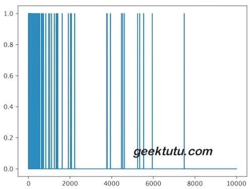
我们这次采用 multi-hot encoding的方式处理 IMDB 数据集,这样能快速达到过拟合的效果。multi-hot 的方式很简单,给每一个单词一个编号,每句话用长度为10,000的一维向量表示,将出现单词的位置置为1即可。
import tensorflow as tffrom tensorflow import kerasfrom tensorflow.keras.datasets import imdbimport numpy as npimport matplotlib.pyplot as plt# 解决中文乱码问题plt.rcParams['font.sans-serif'] = ['SimHei']plt.rcParams['axes.unicode_minus'] = Falseplt.rcParams['font.size'] = 20N = 10000def multi_hot_encoding(sentences, dim=10000):results = np.zeros((len(sentences), dim))for i, word_indices in enumerate(sentences):results[i, word_indices] = 1.0return results(train_x, train_y), (test_x, test_y) = imdb.load_data(num_words=N)train_x = multi_hot_encoding(train_x)test_x = multi_hot_encoding(test_x)plt.plot(train_x[0])plt.show()
如果出现这样的错误,[SSL: CERTIFICATE_VERIFY_FAILED] certificate verify failed: unable to get local issuer certificate (_ssl.c:1045),解决办法可以参考 Github - google-images-download
过拟合
防止过拟合最简单的方式是降低模型复杂度,比如减少模型的学习参数(learnable parameters)。减少神经网络的层数,减少每一层网络的节点数都能达到目的。在深度学习中,学习参数的数量往往代表了模型“容量”(capacity)。容量越大,记忆能力越强,更容易学习到训练集的特征和标签的映射关系,类似于字典。如果这种映射关系缺乏泛化能力,在测试集上不可能有好的表现。
训练的目的不是为了让模型完全拟合训练数据,而是为了训练出具有泛化能力的模型。
反过来,如果模型较小,记忆能力较弱,学习映射关系比较困难。为了最小化损失(loss),模型需要压缩学习到的东西,因而具备更好的预测能力。但是,如果模型过小,没有足够的神经元记住有用的信息,训练会非常困难。因此需要取得权衡。
如何选择合适的网络层数和神经元数量呢?没有公式,只能不断尝试。
为了确定合适的模型大小,建议一开始采用一个参数少的模型,然后逐渐增大,直到验证集的损失(loss)基本不再变化。我们用之前的 IMDB 影评分类模型来试一试。
先搭一个基线模型,再创建大、小2个模型比较。
def build_and_train(hidden_dim, regularizer=None, dropout=0):model = keras.Sequential([keras.layers.Dense(hidden_dim, activation='relu',input_shape=(N,),kernel_regularizer=regularizer),keras.layers.Dropout(dropout),keras.layers.Dense(hidden_dim, activation='relu',kernel_regularizer=regularizer),keras.layers.Dropout(dropout),keras.layers.Dense(1, activation='sigmoid')])model.compile(optimizer='adam', loss='binary_crossentropy',metrics=['accuracy', 'binary_crossentropy'])history = model.fit(train_x, train_y, epochs=10, batch_size=512,validation_data=(test_x, test_y), verbose=0)return historybaseline_history = build_and_train(16)smaller_history = build_and_train(4)larger_history = build_and_train(512)
我们画图看一看这三个模型在训练集和验证集上的表现。
def plot_history(histories, key='binary_crossentropy'):plt.figure(figsize=(10, 6))for name, history in histories:val = plt.plot(history.epoch, history.history['val_'+key],'--', label=name + ' 验证集')plt.plot(history.epoch, history.history[key],color=val[0].get_color(), label=name + ' 训练集')plt.xlabel('Epochs')plt.ylabel('Loss - ' + key)plt.legend()plt.xlim([0, max(history.epoch)])plot_history([('基线', baseline_history),('较小', smaller_history),('较大', larger_history)])
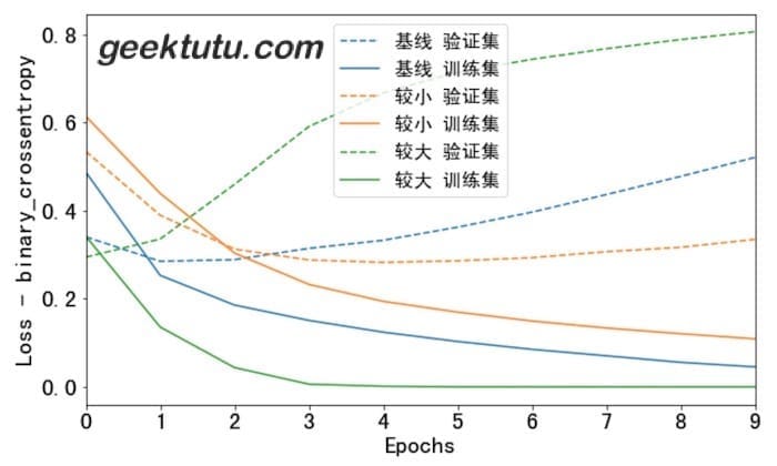
大的模型在第一波(epoch)训练后,就已经过拟合了。模型容量越大,就会越快地拟合训练数据,虽然训练集损失(loss)很低,但事实上已经过拟合了,验证集的loss明显大于训练集。
如何防止过拟合
权重正则化
如果关于同一个问题有许多种理论,每一种都能作出同样准确的预言,那么应该挑选其中使用假定最少的。尽管越复杂的方法通常能做出越好的预言,但是在结果大致相同的情况下,假设越少越好。 —— 维基百科《奥卡剃须刀》
你可能听说过奥卡剃须刀原则——如无必要,勿增实体。将这个原则应用到神经网络模型,相同的预测能力下,优选简单的模型,比起复杂的模型,简单的模型不容易过拟合。
将模型变简单,除了将模型变小(减少网络层数和每层神经元个数)以外,还有另一种方式,减小模型权重(w)的熵(entropy)。即限制权重值在一个较小的范围内,这样模型中权重分布看起来更“regular”,这被称为“权重正则化”(weight regularization)。常用L1正则化和L2正则化2种方式,L2 正则化更通用。
正则化建议参考:机器学习中常常提到的正则化到底是什么意思?
Dropout
在神经网络中,Dropout是最有效的以及使用最广泛的正则化方式。Dropout作用在网络层,训练过程中随机丢弃(dropping out)一部分输出值(例如置为0),Dropout的比例一般置为0.2到0.5之间。例如:
[0.2, 0.3, 0.5, 0.7, 0.9]# after 40% dropout[0.2, 0, 0.5, 0.7, 0]
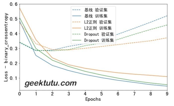
看看效果吧。
l2_model_history = build_and_train(16, keras.regularizers.l2(0.001))dpt_model_history = build_and_train(16, dropout=0.2)plot_history([('基线', baseline_history),('L2正则', l2_model_history),('Dropout', dpt_model_history)])
 )
)
返回文档首页
完整代码:Github - explore_imdb_overfit.ipynb 参考文档:Explore overfitting and underfitting
附 推荐

若有收获,就点个赞吧
0 人点赞
