05.自然语言处理NLTK

01.NLTK (Natural Language Toolkit)
NTLK是著名的Python自然语言处理工具包，但是主要针对的是英文处理。NLTK配套有文档，有语料库，有书籍。
NLP领域中最常用的一个Python库
开源项目
自带分类、分词等功能
强大的社区支持
语料库，语言的实际使用中真是出现过的语言材料
http://www.nltk.org/py-modindex.html
在NLTK的主页详细介绍了如何在Mac、Linux和Windows下安装NLTK：http://nltk.org/install.html ，建议直接下载Anaconda，省去了大部分包的安装，安装NLTK完毕，可以import nltk测试一下，如果没有问题，还有下载NLTK官方提供的相关语料。
安装步骤：
下载NLTK包 pip install nltk
运行Python，并输入下面的指令
import nltk nltk.download()
弹出下面的窗口，建议安装所有的包 ，即all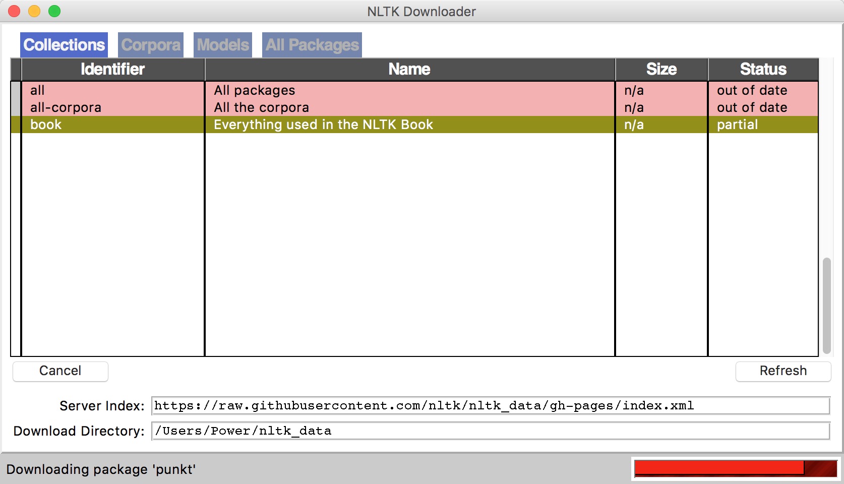

测试使用：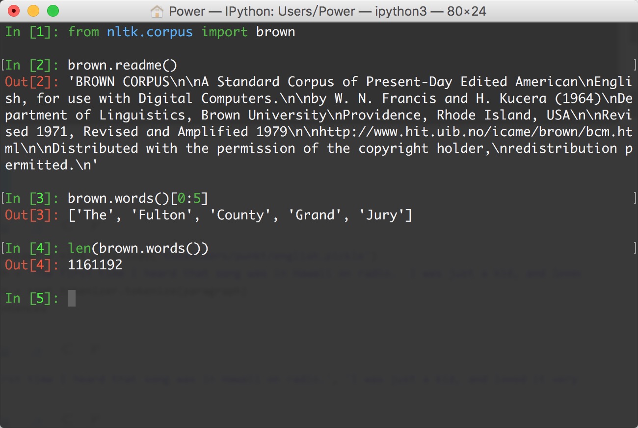

语料库
nltk.corpus
import nltkfrom nltk.corpus import brown # 需要下载brown语料库# 引用布朗大学的语料库# 查看语料库包含的类别print(brown.categories()) # 查看brown语料库print(‘共有{}个句子’.format(len(brown.sents()))) print(‘共有{}个单词’.format(len(brown.words())))
执行结果：
[‘adventure’, ‘belles_lettres’, ‘editorial’, ‘fiction’, ‘government’, ‘hobbies’, ‘humor’, ‘learned’, ‘lore’, ‘mystery’, ‘news’, ‘religion’, ‘reviews’, ‘romance’, ‘science_fiction’] 共有57340个句子 共有1161192个单词
分词 (tokenize)
将句子拆分成具有语言语义学上意义的词
中、英文分词区别：
英文中，单词之间是以空格作为自然分界符的
中文中没有一个形式上的分界符，分词比英文复杂的多
中文分词工具，如：结巴分词 pip install jieba
得到分词结果后，中英文的后续处理没有太大区别
# 导入jieba分词import jieba seg_list = jieba.cut(“欢迎来到黑马程序员Python学科”, cut_all=True) print(“全模式: “ + “/ “.join(seg_list)) # 全模式 seg_list = jieba.cut(“欢迎来到黑马程序员Python学科”, cut_all=False) print(“精确模式: “ + “/ “.join(seg_list)) # 精确模式
运行结果：
全模式: 欢迎/ 迎来/ 来到/ 黑马/ 程序/ 程序员/ Python/ 学科 精确模式: 欢迎/ 来到/ 黑马/ 程序员/ Python/ 学科
词形问题
look, looked, looking
影响语料学习的准确度
词形归一化
1. 词干提取(stemming)
示例：
# PorterStemmerfrom nltk.stem.porter import PorterStemmer porter_stemmer = PorterStemmer() print(porter_stemmer.stem(‘looked’)) print(porter_stemmer.stem(‘looking’)) # 运行结果：# look# look
示例：
# SnowballStemmerfrom nltk.stem import SnowballStemmer snowball_stemmer = SnowballStemmer(‘english’) print(snowball_stemmer.stem(‘looked’)) print(snowball_stemmer.stem(‘looking’)) # 运行结果：# look# look
示例：
# LancasterStemmerfrom nltk.stem.lancaster import LancasterStemmer lancaster_stemmer = LancasterStemmer() print(lancaster_stemmer.stem(‘looked’)) print(lancaster_stemmer.stem(‘looking’)) # 运行结果：# look# look
2. 词形归并(lemmatization)
stemming，词干提取，如将ing, ed去掉，只保留单词主干
lemmatization，词形归并，将单词的各种词形归并成一种形式，如am, is, are -> be, went->go
NLTK中的stemmer
PorterStemmer, SnowballStemmer, LancasterStemmer
NLTK中的lemma
WordNetLemmatizer
问题
went 动词 -> go， 走 Went 名词 -> Went，文特
指明词性可以更准确地进行lemma
示例：
from nltk.stem import WordNetLemmatizer # 需要下载wordnet语料库 wordnet_lematizer = WordNetLemmatizer() print(wordnet_lematizer.lemmatize(‘cats’)) print(wordnet_lematizer.lemmatize(‘boxes’)) print(wordnet_lematizer.lemmatize(‘are’)) print(wordnet_lematizer.lemmatize(‘went’)) # 运行结果：# cat# box# are# went
示例：
# 指明词性可以更准确地进行lemma# lemmatize 默认为名词print(wordnet_lematizer.lemmatize(‘are’, pos=’v’)) print(wordnet_lematizer.lemmatize(‘went’, pos=’v’)) # 运行结果：# be# go
3. 词性标注 (Part-Of-Speech)
NLTK中的词性标注
nltk.word_tokenize()
示例：
import nltk words = nltk.word_tokenize(‘Python is a widely used programming language.’) print(nltk.pos_tag(words)) # 需要下载 averaged_perceptron_tagger# 运行结果：# [(‘Python’, ‘NNP’), (‘is’, ‘VBZ’), (‘a’, ‘DT’), (‘widely’, ‘RB’), (‘used’, ‘VBN’), (‘programming’, ‘NN’), (‘language’, ‘NN’), (‘.’, ‘.’)]
4. 去除停用词
为节省存储空间和提高搜索效率，NLP中会自动过滤掉某些字或词
停用词都是人工输入、非自动化生成的，形成停用词表
分类
语言中的功能词，如the, is…
词汇词，通常是使用广泛的词，如want
中文停用词表
中文停用词库
哈工大停用词表
四川大学机器智能实验室停用词库
百度停用词列表
其他语言停用词表
http://www.ranks.nl/stopwords
使用NLTK去除停用词
stopwords.words()
示例：
from nltk.corpus import stopwords # 需要下载stopwords filtered_words = [word for word in words if word not in stopwords.words(‘english’)] print(‘原始词：’, words) print(‘去除停用词后：’, filtered_words) # 运行结果：# 原始词： [‘Python’, ‘is’, ‘a’, ‘widely’, ‘used’, ‘programming’, ‘language’, ‘.’]# 去除停用词后： [‘Python’, ‘widely’, ‘used’, ‘programming’, ‘language’, ‘.’]
5. 典型的文本预处理流程
示例：
import nltkfrom nltk.stem import WordNetLemmatizerfrom nltk.corpus import stopwords # 原始文本raw_text = ‘Life is like a box of chocolates. You never know what you\’re gonna get.’# 分词raw_words = nltk.word_tokenize(raw_text) # 词形归一化wordnet_lematizer = WordNetLemmatizer() words = [wordnet_lematizer.lemmatize(raw_word) for raw_word in raw_words] # 去除停用词filtered_words = [word for word in words if word not in stopwords.words(‘english’)] print(‘原始文本：’, raw_text) print(‘预处理结果：’, filtered_words)
运行结果：
原始文本： Life is like a box of chocolates. You never know what you’re gonna get. 预处理结果： [‘Life’, ‘like’, ‘box’, ‘chocolate’, ‘.’, ‘You’, ‘never’, ‘know’, “‘re”, ‘gon’, ‘na’, ‘get’, ‘.’]
使用案例：
import nltkfrom nltk.tokenize import WordPunctTokenizer sent_tokenizer = nltk.data.load(‘tokenizers/punkt/english.pickle’) paragraph = “The first time I heard that song was in Hawaii on radio. I was just a kid, and loved it very much! What a fantastic song!” # 分句sentences = sent_tokenizer.tokenize(paragraph) print(sentences) sentence = “Are you old enough to remember Michael Jackson attending. the Grammys with Brooke Shields and Webster sat on his lap during the show?” # 分词words = WordPunctTokenizer().tokenize(sentence.lower()) print(words)
输出结果：
[‘The first time I heard that song was in Hawaii on radio.’, ‘I was just a kid, and loved it very much!’, ‘What a fantastic song!’] [‘are’, ‘you’, ‘old’, ‘enough’, ‘to’, ‘remember’, ‘michael’, ‘jackson’, ‘attending’, ‘.’, ‘the’, ‘grammys’, ‘with’, ‘brooke’, ‘shields’, ‘and’, ‘webster’, ‘sat’, ‘on’, ‘his’, ‘lap’, ‘during’, ‘the’, ‘show’, ‘?’]

02.jieba分词
jieba分词是python写成的一个算是工业界的分词开源库，其github地址为：https://github.com/fxsjy/jieba，在Python里的安装方式： pip install jieba
简单示例：
import jieba as jb seglist = jb.cut(“我来到北京清华大学”, cutall=True) print(“全模式: “ + “/ “.join(seglist)) # 全模式 seglist = jb.cut(“我来到北京清华大学”, cut_all=False) print(“精确模式: “ + “/ “.join(seg_list)) # 精确模式 seg_list = jb.cut(“他来到了网易杭研大厦”) print(“默认模式: “ + “/ “.join(seg_list)) # 默认是精确模式 seg_list = jb.cut_for_search(“小明硕士毕业于中国科学院计算所，后在日本京都大学深造”) print(“搜索引擎模式: “ + “/ “.join(seg_list)) # 搜索引擎模式
执行结果：
全模式: 我/ 来到/ 北京/ 清华/ 清华大学/ 华大/ 大学 精确模式: 我/ 来到/ 北京/ 清华大学 默认模式: 他/ 来到/ 了/ 网易/ 杭研/ 大厦 搜索引擎模式: 小明/ 硕士/ 毕业/ 于/ 中国/ 科学/ 学院/ 科学院/ 中国科学院/ 计算/ 计算所/ ，/ 后/ 在/ 日本/ 京都/ 大学/ 日本京都大学/ 深造
jieba分词的基本思路
jieba分词对已收录词和未收录词都有相应的算法进行处理，其处理的思路很简单，主要的处理思路如下：
加载词典dict.txt
从内存的词典中构建该句子的DAG（有向无环图）
对于词典中未收录词，使用HMM模型的viterbi算法尝试分词处理
已收录词和未收录词全部分词完毕后，使用dp寻找DAG的最大概率路径 输出分词结果
案例：
#!/usr/bin/env python# -- coding:utf-8 --import jiebaimport requestsfrom bs4 import BeautifulSoup def extract_text(url): # 发送url请求并获取响应文件 page_source = requests.get(url).content bs_source = BeautifulSoup(page_source, “lxml”) # 解析出所有的p标签 report_text = bs_source.find_all(‘p’) text = ‘’ # 将p标签里的所有内容都保存到一个字符串里 for p in report_text: text += p.get_text() text += ‘\n’ return text def word_frequency(text): from collections import Counter # 返回所有分词后长度大于等于2 的词的列表 words = [word for word in jieba.cut(text, cut_all=True) if len(word) >= 2] # Counter是一个简单的计数器，统计字符出现的个数 # 分词后的列表将被转化为字典 c = Counter(words) for word_freq in c.most_common(10): word, freq = word_freq print(word, freq) if __name == “__main“: url = ‘http://www.gov.cn/premier/2017-03/16/content_5177940.htm‘ text = extract_text(url) word_frequency(text)
执行结果：
Building prefix dict from the default dictionary … Loading model from cache /var/folders/dp/wxmmld_s7k9gk_5fbhdcr2y00000gn/T/jieba.cache Loading model cost 0.843 seconds. Prefix dict has been built succesfully. 发展 134改革 85经济 71推进 66建设 59社会 49人民 47企业 46加强 46政策 46
流程介绍
首先，我们从网上抓取政府工作报告的全文。我将这个步骤封装在一个名叫extract_text的简单函数中，接受url作为参数。因为目标页面中报告的文本在所有的p元素中，所以我们只需要通过BeautifulSoup选中全部的p元素即可，最后返回一个包含了报告正文的字符串。
然后，我们就可以利用jieba进行分词了。这里，我们要选择全模式分词。jieba的全模式分词，即把句子中所有的可以成词的词语都扫描出来, 速度非常快，但是不能解决歧义。之所以这么做，是因为默认的精确模式下，返回的词频数据不准确。
分词时，还要注意去除标点符号，由于标点符号的长度都是1，所以我们添加一个len(word) >= 2的条件即可。
最后，我们就可以利用Counter类，将分词后的列表快速地转化为字典，其中的键值就是键的出现次数，也就是这个词在全文中出现的次数。

03.情感分析
自然语言处理(NLP)
将自然语言（文本）转化为计算机程序更容易理解的形式
预处理得到的字符串 -> 向量化
经典应用
情感分析
文本相似度
文本分类
简单的情感分析
情感字典（sentiment dictionary）
人工构造一个字典，如： like -> 1, good -> 2, bad -> -1, terrible-> -2
根据关键词匹配
如 AFINN-111： http://www2.imm.dtu.dk/pubdb/views/publication_details.php?id=6010，虽简单粗暴，但很实用
问题：
遇到新词，特殊词等，扩展性较差
使用机器学习模型，nltk.classify
案例：使用机器学习实现
# 简单的例子import nltkfrom nltk.stem import WordNetLemmatizerfrom nltk.corpus import stopwordsfrom nltk.classify import NaiveBayesClassifier text1 = ‘I like the movie so much!’text2 = ‘That is a good movie.’text3 = ‘This is a great one.’text4 = ‘That is a really bad movie.’text5 = ‘This is a terrible movie.’def proc_text(text): “”” 预处处理文本 “”” # 分词 raw_words = nltk.word_tokenize(text) # 词形归一化 wordnet_lematizer = WordNetLemmatizer() words = [wordnet_lematizer.lemmatize(raw_word) for raw_word in raw_words] # 去除停用词 filtered_words = [word for word in words if word not in stopwords.words(‘english’)] # True 表示该词在文本中，为了使用nltk中的分类器 return {word: True for word in filtered_words} # 构造训练样本train_data = [[proc_text(text1), 1], [proc_text(text2), 1], [proc_text(text3), 1], [proc_text(text4), 0], [proc_text(text5), 0]] # 训练模型nb_model = NaiveBayesClassifier.train(train_data) # 测试模型text6 = ‘That is a bad one.’print(nb_model.classify(proc_text(text5)))

04.文本相似度
度量文本间的相似性
使用词频表示文本特征
文本中单词出现的频率或次数
NLTK实现词频统计
文本相似度案例：
import nltkfrom nltk import FreqDist text1 = ‘I like the movie so much ‘text2 = ‘That is a good movie ‘text3 = ‘This is a great one ‘text4 = ‘That is a really bad movie ‘text5 = ‘This is a terrible movie’ text = text1 + text2 + text3 + text4 + text5 words = nltk.word_tokenize(text) freq_dist = FreqDist(words) print(freq_dist[‘is’])# 输出结果：# 4 # 取出常用的n=5个单词n = 5# 构造“常用单词列表”most_common_words = freq_dist.most_common(n) print(most_common_words)# 输出结果：# [(‘a’, 4), (‘movie’, 4), (‘is’, 4), (‘This’, 2), (‘That’, 2)] def lookup_pos(most_common_words): “”” 查找常用单词的位置 “”” result = {} pos = 0 for word in most_common_words: result[word[0]] = pos pos += 1 return result # 记录位置std_pos_dict = lookup_pos(most_common_words) print(std_pos_dict)# 输出结果：# {‘movie’: 0, ‘is’: 1, ‘a’: 2, ‘That’: 3, ‘This’: 4} # 新文本new_text = ‘That one is a good movie. This is so good!’# 初始化向量freq_vec = [0] n# 分词new_words = nltk.word_tokenize(new_text) # 在“常用单词列表”上计算词频for new_word in new_words: if new_word in list(std_pos_dict.keys()): freq_vec[std_pos_dict[new_word]] += 1 print(freq_vec)# 输出结果：# [1, 2, 1, 1, 1]
文本分类
TF-IDF （词频-逆文档频率）
TF, Term Frequency（词频），表示某个词在该文件中出现的次数
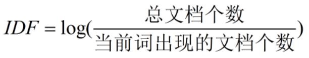
IDF，Inverse Document Frequency（逆文档频率），用于衡量某个词普 遍的重要性。
TF-IDF = TF IDF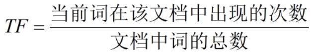

举例假设:
一个包含100个单词的文档中出现单词cat的次数为3，则TF=3/100=0.03
样本中一共有10,000,000个文档，其中出现cat的文档数为1,000个，则IDF=log(10,000,000/1,000)=4
TF-IDF = TF _IDF = 0.03 _4 = 0.12
NLTK实现TF-IDF
TextCollection.tf_idf()
案例：
from nltk.text import TextCollection text1 = ‘I like the movie so much ‘text2 = ‘That is a good movie ‘text3 = ‘This is a great one ‘text4 = ‘That is a really bad movie ‘text5 = ‘This is a terrible movie’# 构建TextCollection对象tc = TextCollection([text1, text2, text3, text4, text5]) new_text = ‘That one is a good movie. This is so good!’word = ‘That’tf_idf_val = tc.tf_idf(word, new_text) print(‘{}的TF-IDF值为：{}’.format(word, tf_idf_val))
执行结果：
That的TF-IDF值为：0.02181644599700369

05.实战案例：微博情感分析
数据：每个文本文件包含相应类的数据

0：喜悦；1：愤怒；2：厌恶；3：低落
步骤
文本读取
分割训练集、测试集
特征提取
模型训练、预测
代码：
tools.py
# -- coding: utf-8 --import reimport jieba.posseg as psegimport pandas as pdimport mathimport numpy as np # 加载常用停用词stopwords1 = [line.rstrip() for line in open(‘./中文停用词库.txt’, ‘r’, encoding=’utf-8’)]# stopwords2 = [line.rstrip() for line in open(‘./哈工大停用词表.txt’, ‘r’, encoding=’utf-8’)]# stopwords3 = [line.rstrip() for line in open(‘./四川大学机器智能实验室停用词库.txt’, ‘r’, encoding=’utf-8’)]# stopwords = stopwords1 + stopwords2 + stopwords3stopwords = stopwords1 def proctext(raw_line): “”” 处理每行的文本数据 返回分词结果 “”” # 1. 使用正则表达式去除非中文字符 filter_pattern = re.compile(‘[^\u4E00-\u9FD5]+’) chinese_only = filter_pattern.sub(‘’, raw_line) # 2. 结巴分词+词性标注 words_lst = pseg.cut(chinese_only) # 3. 去除停用词 meaninful_words = [] for word, flag in words_lst: # if (word not in stopwords) and (flag == ‘v’): # 也可根据词性去除非动词等 if word not in stopwords: meaninful_words.append(word) return ‘ ‘.join(meaninful_words) def split_train_test(text_df, size=0.8): “”” 分割训练集和测试集 “”” # 为保证每个类中的数据能在训练集中和测试集中的比例相同，所以需要依次对每个类进行处理 train_text_df = pd.DataFrame() test_text_df = pd.DataFrame() labels = [0, 1, 2, 3] for label in labels: # 找出label的记录 text_df_w_label = text_df[text_df[‘label’] == label] # 重新设置索引，保证每个类的记录是从0开始索引，方便之后的拆分 text_df_w_label = text_df_w_label.reset_index() # 默认按80%训练集，20%测试集分割 # 这里为了简化操作，取前80%放到训练集中，后20%放到测试集中 # 当然也可以随机拆分80%，20%（尝试实现下DataFrame中的随机拆分） # 该类数据的行数 n_lines = text_df_w_label.shape[0] split_line_no = math.floor(n_lines * size) text_df_w_label_train = text_df_w_label.iloc[:split_line_no, :] text_df_w_label_test = text_df_w_label.iloc[split_line_no:, :] # 放入整体训练集，测试集中 train_text_df = train_text_df.append(text_df_w_label_train) test_text_df = test_text_df.append(text_df_w_label_test) train_text_df = train_text_df.reset_index() test_text_df = test_text_df.reset_index() return train_text_df, test_text_df def get_word_list_from_data(text_df): “”” 将数据集中的单词放入到一个列表中 “”” word_list = [] for , rdata in text_df.iterrows(): word_list += r_data[‘text’].split(‘ ‘) return word_list def extract_feat_from_data(text_df, text_collection, common_words_freqs): “”” 特征提取 “”” # 这里只选择TF-IDF特征作为例子 # 可考虑使用词频或其他文本特征作为额外的特征 n_sample = text_df.shape[0] n_feat = len(common_words_freqs) common_words = [word for word, in commonwordsfreqs] # 初始化 X = np.zeros([nsample, nfeat]) y = np.zeros(n_sample) print(‘提取特征…’) for i, r_data in text_df.iterrows(): if (i + 1) % 5000 == 0: print(‘已完成{}个样本的特征提取’.format(i + 1)) text = r_data[‘text’] feat_vec = [] for word in common_words: if word in text: # 如果在高频词中，计算TF-IDF值 tf_idf_val = text_collection.tf_idf(word, text) else: tf_idf_val = 0 feat_vec.append(tf_idf_val) # 赋值 X[i, :] = np.array(feat_vec) y[i] = int(r_data[‘label’]) return X, y def cal_acc(true_labels, pred_labels): “”” 计算准确率 “”” n_total = len(true_labels) correct_list = [true_labels[i] == pred_labels[i] for i in range(n_total)] acc = sum(correct_list) / n_total return acc
main.py
# main.py# -- coding: utf-8 -- import osimport pandas as pdimport nltkfrom tools import proc_text, split_train_test, get_word_list_from_data, \ extract_feat_from_data, cal_accfrom nltk.text import TextCollectionfrom sklearn.naive_bayes import GaussianNB dataset_path = ‘./dataset’text_filenames = [‘0_simplifyweibo.txt’, ‘1_simplifyweibo.txt’, ‘2_simplifyweibo.txt’, ‘3_simplifyweibo.txt’] # 原始数据的csv文件output_text_filename = ‘raw_weibo_text.csv’# 清洗好的文本数据文件output_cln_text_filename = ‘clean_weibo_text.csv’# 处理和清洗文本数据的时间较长，通过设置is_first_run进行配置# 如果是第一次运行需要对原始文本数据进行处理和清洗，需要设为True# 如果之前已经处理了文本数据，并已经保存了清洗好的文本数据，设为False即可is_first_run = True def read_and_save_to_csv(): “”” 读取原始文本数据，将标签和文本数据保存成csv “”” text_w_label_df_lst = [] for text_filename in text_filenames: text_file = os.path.join(dataset_path, text_filename) # 获取标签，即0, 1, 2, 3 label = int(text_filename[0]) # 读取文本文件 with open(text_file, ‘r’, encoding=’utf-8’) as f: lines = f.read().splitlines() labels = [label] * len(lines) text_series = pd.Series(lines) label_series = pd.Series(labels) # 构造dataframe text_w_label_df = pd.concat([label_series, text_series], axis=1) text_w_label_df_lst.append(text_w_label_df) result_df = pd.concat(text_w_label_df_lst, axis=0) # 保存成csv文件 result_df.columns = [‘label’, ‘text’] result_df.to_csv(os.path.join(dataset_path, output_text_filename), index=None, encoding=’utf-8’) def run_main(): “”” 主函数 “”” # 1. 数据读取，处理，清洗，准备 if is_first_run: print(‘处理清洗文本数据中…’, end=’ ‘) # 如果是第一次运行需要对原始文本数据进行处理和清洗 # 读取原始文本数据，将标签和文本数据保存成csv read_and_save_to_csv() # 读取处理好的csv文件，构造数据集 text_df = pd.read_csv(os.path.join(dataset_path, output_text_filename), encoding=’utf-8’) # 处理文本数据 text_df[‘text’] = text_df[‘text’].apply(proc_text) # 过滤空字符串 text_df = text_df[text_df[‘text’] != ‘’] # 保存处理好的文本数据 text_df.to_csv(os.path.join(dataset_path, output_cln_text_filename), index=None, encoding=’utf-8’) print(‘完成，并保存结果。’) # 2. 分割训练集、测试集 print(‘加载处理好的文本数据’) clean_text_df = pd.read_csv(os.path.join(dataset_path, output_cln_text_filename), encoding=’utf-8’) # 分割训练集和测试集 train_text_df, test_text_df = split_train_test(clean_text_df) # 查看训练集测试集基本信息 print(‘训练集中各类的数据个数：’, train_text_df.groupby(‘label’).size()) print(‘测试集中各类的数据个数：’, test_text_df.groupby(‘label’).size()) # 3. 特征提取 # 计算词频 n_common_words = 200 # 将训练集中的单词拿出来统计词频 print(‘统计词频…’) all_words_in_train = get_word_list_from_data(train_text_df) fdisk = nltk.FreqDist(all_words_in_train) common_words_freqs = fdisk.most_common(n_common_words) print(‘出现最多的{}个词是：’.format(n_common_words)) for word, count in common_words_freqs: print(‘{}: {}次’.format(word, count)) print() # 在训练集上提取特征 text_collection = TextCollection(train_text_df[‘text’].values.tolist()) print(‘训练样本提取特征…’, end=’ ‘) train_X, train_y = extract_feat_from_data(train_text_df, text_collection, common_words_freqs) print(‘完成’) print() print(‘测试样本提取特征…’, end=’ ‘) test_X, test_y = extract_feat_from_data(test_text_df, text_collection, common_words_freqs) print(‘完成’) # 4. 训练模型Naive Bayes print(‘训练模型…’, end=’ ‘) gnb = GaussianNB() gnb.fit(train_X, train_y) print(‘完成’) print() # 5. 预测 print(‘测试模型…’, end=’ ‘) test_pred = gnb.predict(test_X) print(‘完成’) # 输出准确率 print(‘准确率：’, cal_acc(test_y, test_pred)) if __name == ‘__main‘: run_main()