重参数化技巧

http://gregorygundersen.com/blog/2018/04/29/reparameterization/

In Auto-Encoding Variational Bayes, (Kingma & Welling, 2013), Kingma presents an unbiased, differentiable, and scalable estimator for the ELBO in variational inference. A key idea behind this estimator is the reparameterization trick. But why do we need this trick in the first place? When first learning about variational autoencoders (VAEs), I tried to find an answer online but found the explanations too informal. Here are a few examples:

StackExchange: We need the reparameterization trick in order to backpropagate through a random node.

Reddit: The “trick” part of the reparameterization trick is that you make the randomness an input to your model instead of something that happens “inside” it, which means you never need to differentiate with respect to sampling (which you can’t do).

Quora: The problem is because backpropogation cannot flow through a random node.

I found these unsatisfactory. What does a “random node” mean and what does it mean for backprop to “flow” or not flow through such a node?
The goal of this post is to provide a more formal answer for why we need the reparameterization trick. I assume the reader is familiar with variational inference and variational autoencoders. Otherwise, I recommend (Blei et al., 2017) and (Doersch, 2016) as introductions.

Undifferentiable expectations

Let’s say we want to take the gradient w.r.t. of the following expectation,

where pp is a density. Provided we can differentiate , we can easily compute the gradient:

In words, the gradient of the expectation is equal to the expectation of the gradient. But what happens if our density is also parameterized by ?

The first term of the last equation is not guaranteed to be an expectation. Monte Carlo methods require that we can sample from , but not that we can take its gradient. This is not a problem if we have an analytic solution to , but this is not true in general.
Now that we have a better understanding of the problem, let’s see what happens when we apply the reparameterization trick to our simple example. To be consistent with Kingma, I’ll switch to bold text for vectors and denote the ii_th sample of vector as and to denote the l_l_th Monte Carlo sample:

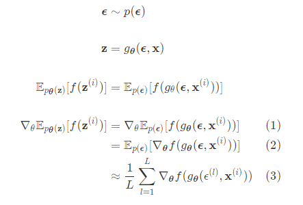
In my mind, the above line of reasoning is key to understanding VAEs. We use the reparameterization trick to express a gradient of an expectation (1) as an expectation of a gradient (2). Provided  is differentiable—something Kingma emphasizes—then we can then use Monte Carlo methods to estimate (3).

Sanity check

It is worth noting that this explanation aligns with Kingma’s own justification:

Kingma: This reparameterization is useful for our case since it can be used to rewrite an expectation w.r.t such that the Monte Carlo estimate of the expectation is differentiable w.r.t. .

The issue is not that we cannot backprop through a “random node” in any technical sense. Rather, backproping would not compute an estimate of the derivative. Without the reparameterization trick, we have no guarantee that sampling large numbers of \textbf{z}z will help converge to the right estimate of \nabla{\theta}∇θ_.
Furthermore, this is the exact problem we have with the ELBO we want to estimate:

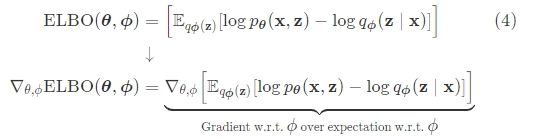
At this point, you might have noticed that the above equation does not look like what we compute in a standard VAE. In the paper, Kingma actually presents two estimators, which he denotes and . Equation (4)(4) is , while \mathcal{L}^BLB is an estimator we can use when we have an analytic solution to the KL-divergence term in the ELBO, for example when we assume both the prior p{\boldsymbol{\theta}}(\textbf{z})_pθ(z) and the posterior approximation q{\boldsymbol{\phi}}(\textbf{z} \mid \textbf{x})_qϕ(z∣x) are Gaussian:

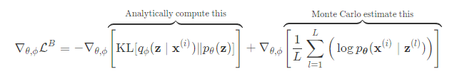
Now that we can compute the full loss through a sequence of differentiable operations, we can use our favorite gradient-based optimization technique to maximize the ELBO.

Implementation

I always find it useful to close the loop and talk about implementation. The equation above is what the standard VAE implements (example) because Kingma derives an analytic solution for the KL term in Appendix 2. A common framing for this version of the model is to think of the likelihood as a “decoder” and the approximate posterior as an “encoder”:
\mathcal{L}^B = - \text{KL}[\overbrace{q{\phi}(\textbf{z} \mid \textbf{x}^{(i)})}^{\text{Encoder}} \lVert \overbrace{p{\theta}(\textbf{z})}^{\text{Fixed}}] + \frac{1}{L} \sum{l=1}^{L} \log \overbrace{p{\boldsymbol{\theta}}(\textbf{x}^{(i)} \mid \textbf{z}^{(l)})}^{\text{Decoder}}LB=−KL[q__ϕ(z∣x(i))Encoder∥p__θ(z)Fixed]+L_1_l=1∑L_log_pθ(x(i)∣z(l))Decoder
I think of it like this: the KL-divergence term encourages the approximate posterior to be close to the prior p{\boldsymbol{\theta}}(\textbf{z})_pθ(z). If the approximate posterior could exactly match both the real posterior and the prior, then using Bayes’ rule we would know that p(\textbf{x}) = p(\textbf{x} \mid \textbf{z})p(x)=p(x∣z). This is exactly what we would want from a generative model. We could sample \textbf{z}z using the reparameterization trick and then condition on \textbf{z}z to generate a realistic sample \textbf{x}x.
Concretely, here is one pass through the computational graph when the prior and approximate posterior are Gaussian:
μx,σxϵzxrrecon. lossvar. lossL=M(x),Σ(x)∼N(0,1)=ϵσx+μx=pθ(x∣z)=MSE(x,xr)=−KL[N(μx,σx)∥N(0,I)]=recon. loss+var. lossPush x through encoderSample noiseReparameterizePush z through decoderCompute reconstruction lossCompute variational lossCombine lossesμx,σx=M(x),Σ(x)Push x through encoderϵ∼N(0,1)Sample noisez=ϵσx+μxReparameterizexr=pθ(x∣z)Push z through decoderrecon. loss=MSE(x,xr)Compute reconstruction lossvar. loss=−KL[N(μx,σx)‖N(0,I)]Compute variational lossL=recon. loss+var. lossCombine losses
μx,σxϵzxr_recon. lossvar. lossL=_M(x),Σ(x)∼N(0,1)=ϵσx+μx=pθ(x∣z)=MSE(x,xr)=−KL[N(μx,σx)∥N(0,I)]=recon. loss+var. lossPush x through encoderSample noiseReparameterizePush z through decoderCompute reconstruction lossCompute variational lossCombine losses
Since we computed every variable in this computational graph through a sequence of differentiable operations, we can use a method like backpropagation to compute the required gradients. I find this easiest to see via a diagram: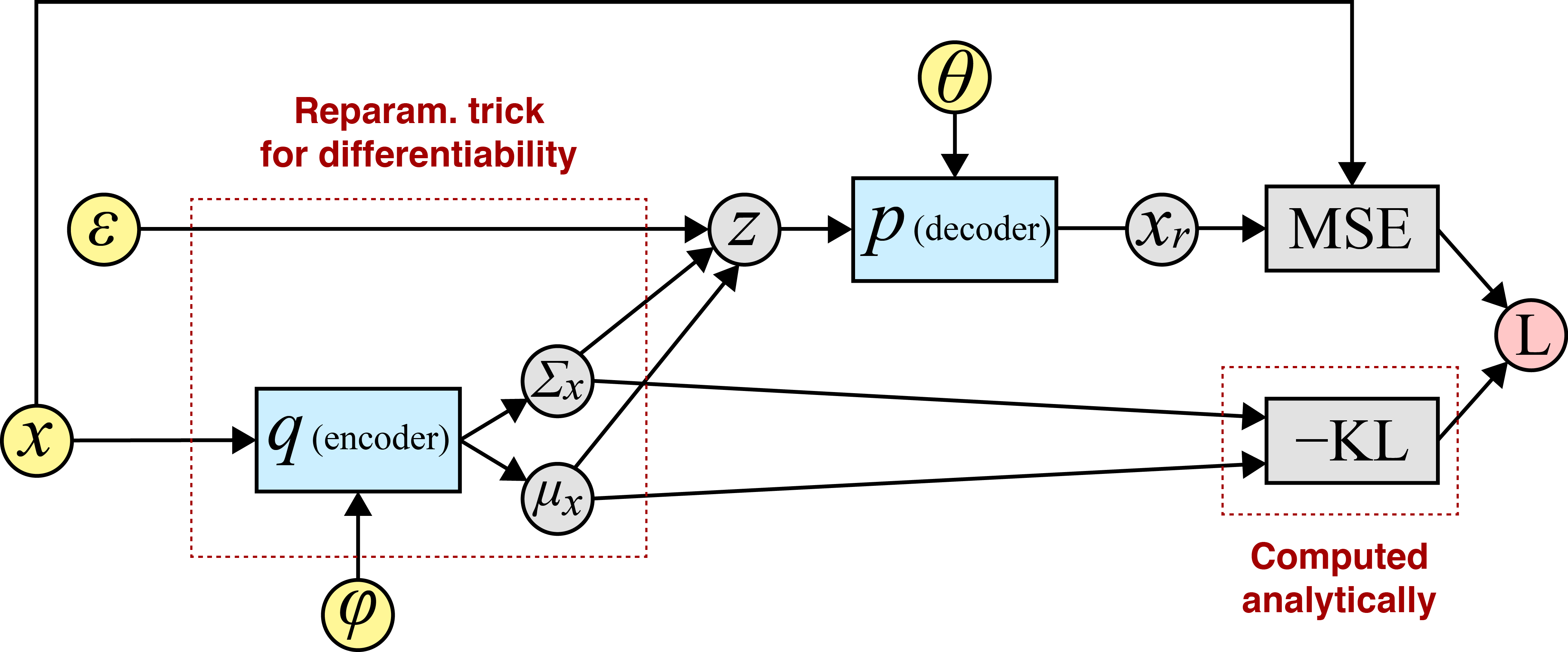

Above, the input or root nodes are in yellow. I like to denote the network parameters as inputs because it emphasizes how a tool like autograd (Maclaurin et al., 2015) actually works: for a given parameter ww, we can compute \partial L / \partial w∂L/∂w at the graph node that directly takes ww as input.

What’s in a name?

When I first read Kingma’s paper, I wondered why it focused on the stochastic gradient variational Bayes (SGVB) estimator and associated algorithm, while the now-famous variational autoencoder was just given as an example halfway through the paper.
But with a better understanding of the differentiability of this Monte Carlo estimator, we can understand the focus of the paper and the name of the estimator. Variational Bayes refers to approximating integrals using Bayesian inference. The method is stochastic because it approximates an expectation with many random samples. And a VAE using neural networks is an example of a model you could build with the SGVB estimator because the estimator is gradient-based.