6 CONCURRENCY IN NETWORKS 网络中的并发

The high average parallelism (W/D) in neural networks may not only be harnessed to compute individual operators efficiently, but also to evaluate the whole network concurrently with respect to different dimensions.
神经网络中的高平均并行性 (W/D) 不仅可以用于有效地计算单个算子，还可以针对不同维度同时评估整个网络。

Owing to the use of minibatches, the breadth (∝ W) of the layers, and the depth of the DNN (∝ D), it is possible to partition both the forward evaluation and the backpropagation phases (lines 4–5 in Algorithm 2) among parallel processors.
由于使用了小批量，层的宽度 (∝ W) 和DNN的深度(∝ D)，可以在并行处理器之间划分正向评估和反向传播阶段 (算法2中的第4-5行)。

Below, we discuss three prominent partitioning strategies, illustrated in Fig. 14: partitioning by input samples (data parallelism), by network structure (model parallelism), and by layer (pipelining).
下面，我们讨论三种突出的分区策略，如图14所示: 按输入样本 (数据并行性) 、按网络结构 (模型并行性) 和按层 (流水线) 进行分区。

6.1 Data Parallelism

In minibatch SGD (Section 2.1.2), data is processed in increments of N samples.
在minibatch SGD (第2.1.2节) 中，以N个样本为增量处理数据。

As most of the operators are independent with respect to N (Section 4), a straightforward approach for parallelization is to partition the work of the minibatch samples among multiple computational resources (cores or devices).
由于大多数运算符相对于N是独立的 (第4节)，并行化的一种简单方法是在多个计算资源 (核心或设备) 之间划分小批量样本的工作。

This method (initially named pattern parallelism, as input samples were called patterns), dates back to the first practical implementations of artificial neural networks[262].
这种方法 (最初命名为模式并行性，因为输入样本被称为模式) 可以追溯到人工神经网络的第一个实际实现 [262]。

It could be argued that the use of minibatches in SGD for neural networks was initially driven by data parallelism.
可以认为，在SGD中使用微型批次用于神经网络最初是由数据并行性驱动的。

Farber and Asanović[73] used multiple vector accelerator microprocessors (Spert-II) to parallelize error backpropagation for neural network training.
Farber和asanovi ic [73] 使用多矢量加速器微处理器 (Spert-II) 并行化误差反向传播，用于神经网络训练。

To support data parallelism, the paper presents a version of delayed gradient updates called “bunch mode”, where the gradient is updated several times prior to updating the weights, essentially equivalent to minibatch SGD.
为了支持数据并行性，本文提出了一种称为 “束模式” 的延迟梯度更新版本，其中梯度在更新权重之前更新了几次，基本上相当于minibatch SGD。

One of the earliest occurrences of mapping DNN computations to data parallel architectures (e.g., GPUs) were performed by Raina et al.[200].
将DNN计算映射到数据并行架构 (如图形处理器) 的最早出现之一是由吴慧琳等人完成的 [200]。

The paper focuses on the problem of training Deep Belief Networks[97], mapping the unsupervised training procedure to GPUs by running minibatch SGD.
本文主要研究训练深度信念网络的问题 [97]，通过运行minibatch SGD将无监督训练过程映射到gpu。

The paper shows speedup of up to 72.6× over CPU when training Restricted Boltzmann Machines.
本文显示，当训练受限的玻尔兹曼机器时，CPU的加速速度高达72.6倍。

Today, data parallelism is supported by the vast majority of deep learning frameworks, using a single GPU, multiple GPUs, or a cluster of multi-GPU nodes.
如今，绝大多数深度学习框架都支持数据并行性，它们使用单个GPU、多个GPU或多个GPU节点集群。

The scaling of data parallelism is naturally defined by the minibatch size (Table 4).
数据并行性的缩放自然由minibatch大小定义 (表4)。

Apart from Batch Normalization (BN)[117], all operators mentioned in Section 4 operate on a single sample at a time, so forward evaluation and backpropagation are almost completely independent.
除了批量标准化 (BN)[117]，第4节中提到的所有运算符一次对单个样本进行操作，因此正向评估和反向传播几乎是完全独立的。

In the weight update phase, however, the results of the partitions have to be averaged to obtain the gradient w.r.t. the whole minibatch, which potentially induces an allreduce operation.
然而，在权重更新阶段，必须对分区的结果进行平均以获得梯度w.r.t.整个微型批处理，可能会引发allcut操作。

Furthermore, in this partitioning method, all DNN parameters have to be accessible for all participating devices, which means that they should be replicated.
此外，在此分区方法中，所有参与设备都必须可访问所有DNN参数，这意味着应复制它们。

6.1.1 Neural Architecture Support for Large Minibatches. 支持大型小批量的神经架构。

……

6.2 Model Parallelism

The second partitioning strategy for DNN training is model parallelism (also known as network parallelism).
DNN训练的第二种分区策略是模型并行性 (也称为网络并行性)。

This strategy divides the work according to the neurons in each layer, namely the C, H, or W dimensions in a 4-dimensional tensor.
这种策略根据每一层中的神经元来划分工作，即4维张量中的C、H或W维。

In this case, the sample minibatch is copied to all processors, and different parts of the DNN are computed on different processors, which can conserve memory (since the full network is not stored in one place) but incurs additional communication after every layer.
在这种情况下，将示例minibatch复制到所有处理器，并在不同的处理器上计算DNN的不同部分，这可以节省内存 (因为整个网络不存储在一个地方)，但在每一层之后会产生额外的通信。

Since the minibatch size does not change in model parallelism, the utilization vs. generalization tradeoff (Section 3) does not apply.
由于微型批处理大小在模型并行性中没有变化，因此利用率与泛化权衡 (第3节) 不适用。

Nevertheless, the DNN architecture creates layer interdependencies, which, in turn, generate communication that determines the overall performance.
然而，DNN体系结构创建层相互依赖关系，进而生成决定整体性能的通信。

Fully connected layers, for instance, incur all-to-all communication (as opposed to allreduce in data parallelism), as neurons connect to all the neurons of the next layer.
例如，当神经元连接到下一层的所有神经元时，全连接层会产生所有到所有的通信 (与数据并行性中的所有减少相反)。

To reduce communication costs in fully connected layers, it has been proposed[174] to introduce redundant computations to neural networks.
为了降低完全连接层的通信成本，已经提出 [174] 将冗余计算引入神经网络。

In particular, the proposed method partitions an NN such that each processor will be responsible for twice the neurons (with overlap), and thus would need to compute more but communicate less.
特别地，所提出的方法划分了一个NN，使得每个处理器将负责两倍的神经元 (具有重叠)，因此将需要计算更多但通信更少。

Another method proposed for reducing communication in fully connected layers is to use Cannon’s matrix multiplication algorithm, modified for DNNs[72].
为减少全连接层中的通信而提出的另一种方法是使用坎农矩阵乘法算法，该算法针对DNNs进行了修改 [72]。

The paper reports that Cannon’s algorithm produces better efficiency and speedups over simple partitioning on small-scale multilayer fully connected networks.
本文报告了坎农算法在小型多层全连接网络上比简单分区产生更好的效率和速度。

As for CNNs, using model parallelism for convolutional operators is relatively inefficient.
至于CNNs，对卷积算子使用模型并行性是相对低效的。

If samples are partitioned across processors by feature (channel), then each convolution would have to obtain all results from the other processors to compute its result, as the operation sums over all features.
如果样本通过特征 (通道) 在处理器之间进行分区，那么每个卷积必须从其他处理器获得所有结果来计算其结果，因为操作对所有特征求和。

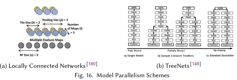
To mitigate this problem, Locally Connected Networks (LCNs)[180] were introduced.
为了缓解这个问题，引入了本地连接网络 (LCNs)[180]。

While still performing convolutions, LCNs define multiple local filters for each region (Fig. 16a), enabling partitioning by the C,H,W dimensions that does not incur all-to-all communication.
当仍然执行卷积时，LCNs为每个区域定义多个局部滤波器 (图16a)，通过C、H、W维度实现分区，不会产生全到全通信。

Using LCNs and model parallelism, thework presented by Coates et al.[45] managed to outperform a CNN of the same size running on 5,000 CPU nodes with a 3-node multi-GPU cluster.
使用LCNs和模型并行性，由Coates等人 [45] 提出的工作成功地超越了在5,000个CPU节点和一个3节点多GPU集群上运行的相同大小的CNN。

Due to the lack of weight sharing (apart from spatial image boundaries), training is not communication-bound,
and scaling can be achieved.
由于重量分担的缺乏 (除了空间图像边界)，训练不局限于交流，并且可以实现缩放。

Successfully applying the same techniques on CNNs requires finegrained control over parallelism, as we shall show in Section 6.4.
在CNNs上成功应用相同的技术需要对并行性进行细粒度控制，正如我们将在第6.4节中展示的那样。

Unfortunately, weight sharing is an important part of CNNs, contributing to memory footprint reduction as well as improving generalization, and thus standard convolutional operators are used more frequently than LCNs.
不幸的是，权重共享是CNNs的重要组成部分，有助于减少内存占用以及改善泛化，因此标准卷积算子比LCNs使用得更频繁。

A second form of model parallelism is the replication of DNN elements.
模型并行性的第二种形式是DNN元素的复制。

In TreeNets[148], the authors study ensembles of DNNs (groups of separately trained networks whose results are averaged, rather than their parameters), and propose a mid-point between ensembles and training a single
model: a certain layer creates a “junction”, from which multiple copies of the network are trained (see Fig. 16b).
在TreeNets[148] 中，作者研究了DNNs的集合 (由单独训练的网络组成的组，其结果是平均的，而不是它们的参数)，并在合奏和训练之间提出一个中点模型: 某一层创建一个 “结点”，从中训练网络的多个副本 (见图16b)。

The paper defines ensemble-aware loss functions and backpropagation techniques, so as to regularize the training process.
本文定义了集成感知损失函数和反向传播技术，以规范训练过程。

The training process, in turn, is parallelized across the network copies, assigning each copy to a different processor.
反过来，训练过程通过网络副本并行化，将每个副本分配给不同的处理器。

The results presented in the paper for three datasets indicate that TreeNets essentially train an ensemble of expert DNNs.
本文针对三个数据集提出的结果表明，树网本质上训练了一组专家DNNs。

6.3 Pipelining

In deep learning, pipelining can either refer to overlapping computations, i.e., between one layer and the next (as data becomes ready); or to partitioning the DNN according to depth, assigning layers to specific processors (Fig. 14c).
在深度学习中，流水线可以指重叠计算，即在一层和下一层之间 (当数据准备就绪时); 或者根据深度对DNN进行分区，将层分配给特定的处理器 (图14c)。

Pipelining can be viewed as a form of data parallelism, since elements (samples) are processed through the network in parallel, but also as model parallelism, since the length of the pipeline is determined by the DNN structure.
流水线可以看作是数据并行性的一种形式，因为元素 (样本) 通过网络并行处理，也可以看作模型并行性，因为管道的长度由DNN结构决定。

The first form of pipelining can be used to overlap forward evaluation, backpropagation, and weight updates.
第一种流水线形式可用于重叠前向评估、反向传播和权重更新。

This scheme is widely used in practice[1,48,119], and increases utilization by mitigating processor idle time.
该方案在实践中被广泛使用 [1,48,119]，并通过减少处理器空闲时间来提高利用率。

In a finer granularity, neural network architectures can be designed around the principle of overlapping layer computations, as is the case with Deep Stacking Networks (DSN)[62].
在更精细的粒度中，可以围绕重叠层计算原理设计神经网络体系结构，就像深度堆叠网络 (DSN) 一样 [62]。

In DSNs, each step computes a different fully connected layer of the data.
在DSNs中，每个步骤计算不同的完全连接的数据层。

However, the results of all previous steps are concatenated to the layer inputs (see Fig. 17a).
然而，所有先前步骤的结果与层输入串联 (见图17a)。

This enables each layer to be partially computed in parallel, due to the relaxed data dependencies.
由于宽松的数据依赖关系，这使得每个层能够部分并行计算。

As for layer partitioning, there are several advantages for a multi-processor pipeline over both data and model parallelism: (a) there is no need to store all parameters on all processors during forward evaluation and backpropagation (as with model parallelism); (b) there is a fixed number of communication points between processors (at layer boundaries), and the source and destination processors are always known.
至于层分区，多处理器管道在数据和模型并行性方面有几个优点 :( a) 在正向评估和反向传播期间，不需要在所有处理器上存储所有参数 (如模型并行性); (b) 处理器之间有固定数量的通信点(在层边界处)，并且源处理器和目标处理器始终是已知的。

Moreover, since the processors always compute the same layers, the weights can remain cached to decrease memory round-trips.
此外，由于处理器总是计算相同的层，权重可以保持缓存以减少内存往返。

Two disadvantages of pipelining, however, are that data (samples) have to arrive at a specific rate in order to fully utilize the system, and that latency proportional to the number of processors is incurred.
然而，流水线的两个缺点是，为了充分利用系统，数据 (样本) 必须以特定的速率到达，并且会产生与处理器数量成比例的延迟。

In the following section,we discuss two implementations of layer partitioning—DistBelief[56] and Project Adam[39] — which combine the advantages of pipelining with data and model parallelism.
在下一节中，我们将讨论层划分的两种实现方式-distfaith [56] 和亚当 [39] -它们结合了流水线与数据和模型并行性的优势。

6.4 Hybrid Parallelism 混合并行性

The combination of multiple parallelism schemes can overcome the drawbacks of each scheme.
多个并行方案的组合可以克服每个方案的缺点。

Below we overview successful instances of such hybrids.
下面我们概述了这种杂交品种的成功实例。

In AlexNet, most of the computations are performed in the convolutional layers, but most of the parameters belong to the fully connected layers.
在AlexNet中，大多数计算是在卷积层中执行的，但是大多数参数属于完全连接的层。

When mapping AlexNet to a multi-GPU node using data or model parallelism separately, the best reported speed up for 4 GPUs over one is ∼2.2×[246].
当单独使用数据或模型并行性将AlexNet映射到多GPU节点时，报告的4个GPU的最佳加速速度为〜2.2 ×[246]。

One successful example[135] of a hybrid scheme applies data parallelism to the convolutional layer, and model parallelism to the fully connected part (see Fig. 17b).
一个混合方案的成功例子 [135] 将数据并行性应用到卷积层，将模型并行性应用到完全连接的部分 (见图17b)。

Using this hybrid approach, a speedup of up to 6.25× can be achieved for 8 GPUs over one, with less than 1% accuracy loss (due to an increase in minibatch size).
使用这种混合方法，8个图形处理器的加速可达6.25倍，精度损失不到1% (由于微型批处理大小的增加)。

These results were also reaffirmed in other hybrid implementations[16], in which 3.1× speedup was achieved for 4 GPUs using the same approach, and derived theoretically using communication cost analysis[77], promoting 1.5D matrix multiplication algorithms for integrated data/model parallelism.
这些结果也在其他混合实现中得到重申 [16]，其中使用相同的方法实现了4个图形处理器的3.1倍加速，并使用通信成本分析从理论上推导 [77]，推广用于集成数据/模型并行性的1.5D矩阵乘法算法。

AMPNet[76] is an asynchronous implementation of DNN training on CPUs, which uses an intermediate representation to implement fine-grained model parallelism.
AMPNet[76] 是cpu上DNN训练的异步实现，它使用中间表示来实现精细的模型并行性。

In particular, internal parallel tasks within and between layers are identified and scheduled asynchronously.
特别是，层内和层之间的内部并行任务是异步识别和调度的。

Additionally, asynchronous execution of dynamic control flow enables pipelining the tasks of forward evaluation, backpropagation, and weight update (Fig. 15a, right).
此外，动态控制流的异步执行使前向评估、反向传播和权重更新的任务能够流水线化 (图15a，右)。

The main advantage of AMPNet is in recurrent, tree-based, and gated-graph neural networks, all of which exhibit heterogeneous characteristics, i.e., variable length for each sample and dynamic control flow (as opposed to homogeneous CNNs).
AMPNet的主要优势在于递归的、基于树的和门控图神经网络，所有这些都表现出异构特征，即，每个样品和动态控制流的可变长度 (与均匀CNNs相反)。

The paper shows speedups of up to 3.94× over the TensorFlow[1] framework.
本文显示了TensorFlow[1] 框架上高达3.94 × 的加速。

Lastly, the DistBelief[56] distributed deep learning system combines all three parallelism strategies.
最后，DistBelief[56] 分布式深度学习系统结合了所有三种并行策略。

In the implementation, training is performed on multiple model replicas simultaneously, where each replica is trained on different samples (data parallelism).
在实现中，对多个模型副本同时执行训练，其中每个副本都针对不同的样本进行训练 (数据并行性)。

Within each replica (shown in Fig.17c), the DNN is distributed both according to neurons in the same layer (model parallelism), and according to the different layers (pipelining).
在每个副本中 (如图17c所示)，DNN根据同一层中的神经元 (模型并行性) 和不同层 (流水线) 分布。

Project Adam[39] extends upon the ideas of DistBelief and exhibits the same types of parallelism. However, in Project Adam pipelining is restricted to different CPU cores on the same node.
亚当项目 [39] 扩展了疏远思想，并展示了相同类型的排比。然而，亚当流水线仅限于同一节点上的不同CPU内核。