Task2 数据分析

此部分为零基础入门金融风控的 Task2 数据分析部分，带你来了解数据，熟悉数据，为后续的特征工程做准备，欢迎大家后续多多交流。

赛题：零基础入门数据挖掘 - 零基础入门金融风控之贷款违约

目的：

• 1.EDA价值主要在于熟悉了解整个数据集的基本情况（缺失值，异常值），对数据集进行验证是否可以进行接下来的机器学习或者深度学习建模.
• 2.了解变量间的相互关系、变量与预测值之间的存在关系。
• 3.为特征工程做准备

项目地址：https://github.com/datawhalechina/team-learning-data-mining/tree/master/FinancialRiskControl

比赛地址：https://tianchi.aliyun.com/competition/entrance/531830/introduction

2.1 学习目标

• 学习如何对数据集整体概况进行分析，包括数据集的基本情况（缺失值，异常值）
• 学习了解变量间的相互关系、变量与预测值之间的存在关系
• 完成相应学习打卡任务

2.2 内容介绍

• 数据总体了解：
  • 读取数据集并了解数据集大小，原始特征维度；
  • 通过info熟悉数据类型；
  • 粗略查看数据集中各特征基本统计量；
• 缺失值和唯一值：
  • 查看数据缺失值情况
  • 查看唯一值特征情况
• 深入数据-查看数据类型
  • 类别型数据
  • 数值型数据
    • 离散数值型数据
    • 连续数值型数据
• 数据间相关关系
  • 特征和特征之间关系
  • 特征和目标变量之间关系
• 用pandas_profiling生成数据报告

2.3 代码示例

2.3.1 导入数据分析及可视化过程需要的库

import pandas as pd
import numpy as np
import matplotlib.pyplot as plt
import seaborn as sns
import datetime
import warnings
warnings.filterwarnings('ignore')

/Users/exudingtao/opt/anaconda3/lib/python3.7/site-packages/statsmodels/tools/_testing.py:19: FutureWarning: pandas.util.testing is deprecated. Use the functions in the public API at pandas.testing instead.
  import pandas.util.testing as tm

以上库都是pip install 安装就好，如果本机有python2,python3两个python环境傻傻分不清哪个的话,可以pip3 install 。或者直接在notebook中’!pip3 install ‘安装。

说明：

本次数据分析探索，尤其可视化部分均选取某些特定变量进行了举例，所以它只是一个方法的展示而不是整个赛题数据分析的解决方案。

2.3.2 读取文件

data_train = pd.read_csv('./train.csv')

data_test_a = pd.read_csv('./testA.csv')

2.3.2.1读取文件的拓展知识

• pandas读取数据时相对路径载入报错时，尝试使用os.getcwd()查看当前工作目录。
• TSV与CSV的区别：
  • 从名称上即可知道，TSV是用制表符（Tab,’\t’）作为字段值的分隔符；CSV是用半角逗号（’,’）作为字段值的分隔符；
  • Python对TSV文件的支持：
    Python的csv模块准确的讲应该叫做dsv模块，因为它实际上是支持范式的分隔符分隔值文件（DSV，delimiter-separated values）的。
    delimiter参数值默认为半角逗号，即默认将被处理文件视为CSV。当delimiter=’\t’时，被处理文件就是TSV。
• 读取文件的部分（适用于文件特别大的场景）
  • 通过nrows参数，来设置读取文件的前多少行，nrows是一个大于等于0的整数。
  • 分块读取

data_train_sample = pd.read_csv("./train.csv",nrows=5)

#设置chunksize参数，来控制每次迭代数据的大小
chunker = pd.read_csv("./train.csv",chunksize=5)
for item in chunker:
    print(type(item))
    #<class 'pandas.core.frame.DataFrame'>
    print(len(item))
    #5

2.3.3总体了解

查看数据集的样本个数和原始特征维度

data_test_a.shape

(200000, 48)

data_train.shape

(800000, 47)

data_train.columns

Index(['id', 'loanAmnt', 'term', 'interestRate', 'installment', 'grade',
       'subGrade', 'employmentTitle', 'employmentLength', 'homeOwnership',
       'annualIncome', 'verificationStatus', 'issueDate', 'isDefault',
       'purpose', 'postCode', 'regionCode', 'dti', 'delinquency_2years',
       'ficoRangeLow', 'ficoRangeHigh', 'openAcc', 'pubRec',
       'pubRecBankruptcies', 'revolBal', 'revolUtil', 'totalAcc',
       'initialListStatus', 'applicationType', 'earliesCreditLine', 'title',
       'policyCode', 'n0', 'n1', 'n2', 'n2.1', 'n4', 'n5', 'n6', 'n7', 'n8',
       'n9', 'n10', 'n11', 'n12', 'n13', 'n14'],
      dtype='object')

查看一下具体的列名，赛题理解部分已经给出具体的特征含义，这里方便阅读再给一下：

• id 为贷款清单分配的唯一信用证标识
• loanAmnt 贷款金额
• term 贷款期限（year）
• interestRate 贷款利率
• installment 分期付款金额
• grade 贷款等级
• subGrade 贷款等级之子级
• employmentTitle 就业职称
• employmentLength 就业年限（年）
• homeOwnership 借款人在登记时提供的房屋所有权状况
• annualIncome 年收入
• verificationStatus 验证状态
• issueDate 贷款发放的月份
• purpose 借款人在贷款申请时的贷款用途类别
• postCode 借款人在贷款申请中提供的邮政编码的前3位数字
• regionCode 地区编码
• dti 债务收入比
• delinquency_2years 借款人过去2年信用档案中逾期30天以上的违约事件数
• ficoRangeLow 借款人在贷款发放时的fico所属的下限范围
• ficoRangeHigh 借款人在贷款发放时的fico所属的上限范围
• openAcc 借款人信用档案中未结信用额度的数量
• pubRec 贬损公共记录的数量
• pubRecBankruptcies 公开记录清除的数量
• revolBal 信贷周转余额合计
• revolUtil 循环额度利用率，或借款人使用的相对于所有可用循环信贷的信贷金额
• totalAcc 借款人信用档案中当前的信用额度总数
• initialListStatus 贷款的初始列表状态
• applicationType 表明贷款是个人申请还是与两个共同借款人的联合申请
• earliesCreditLine 借款人最早报告的信用额度开立的月份
• title 借款人提供的贷款名称
• policyCode 公开可用的策略代码=1新产品不公开可用的策略代码=2
• n系列匿名特征 匿名特征n0-n14，为一些贷款人行为计数特征的处理

通过info()来熟悉数据类型

data_train.info()

<class 'pandas.core.frame.DataFrame'>
RangeIndex: 800000 entries, 0 to 799999
Data columns (total 47 columns):
 #   Column              Non-Null Count   Dtype  
---  ------              --------------   -----  
 0   id                  800000 non-null  int64  
 1   loanAmnt            800000 non-null  float64
 2   term                800000 non-null  int64  
 3   interestRate        800000 non-null  float64
 4   installment         800000 non-null  float64
 5   grade               800000 non-null  object 
 6   subGrade            800000 non-null  object 
 7   employmentTitle     799999 non-null  float64
 8   employmentLength    753201 non-null  object 
 9   homeOwnership       800000 non-null  int64  
 10  annualIncome        800000 non-null  float64
 11  verificationStatus  800000 non-null  int64  
 12  issueDate           800000 non-null  object 
 13  isDefault           800000 non-null  int64  
 14  purpose             800000 non-null  int64  
 15  postCode            799999 non-null  float64
 16  regionCode          800000 non-null  int64  
 17  dti                 799761 non-null  float64
 18  delinquency_2years  800000 non-null  float64
 19  ficoRangeLow        800000 non-null  float64
 20  ficoRangeHigh       800000 non-null  float64
 21  openAcc             800000 non-null  float64
 22  pubRec              800000 non-null  float64
 23  pubRecBankruptcies  799595 non-null  float64
 24  revolBal            800000 non-null  float64
 25  revolUtil           799469 non-null  float64
 26  totalAcc            800000 non-null  float64
 27  initialListStatus   800000 non-null  int64  
 28  applicationType     800000 non-null  int64  
 29  earliesCreditLine   800000 non-null  object 
 30  title               799999 non-null  float64
 31  policyCode          800000 non-null  float64
 32  n0                  759730 non-null  float64
 33  n1                  759730 non-null  float64
 34  n2                  759730 non-null  float64
 35  n2.1                759730 non-null  float64
 36  n4                  766761 non-null  float64
 37  n5                  759730 non-null  float64
 38  n6                  759730 non-null  float64
 39  n7                  759730 non-null  float64
 40  n8                  759729 non-null  float64
 41  n9                  759730 non-null  float64
 42  n10                 766761 non-null  float64
 43  n11                 730248 non-null  float64
 44  n12                 759730 non-null  float64
 45  n13                 759730 non-null  float64
 46  n14                 759730 non-null  float64
dtypes: float64(33), int64(9), object(5)
memory usage: 286.9+ MB

总体粗略的查看数据集各个特征的一些基本统计量

data_train.describe()

data_train.head(3).append(data_train.tail(3))

2.3.4查看数据集中特征缺失值，唯一值等

查看缺失值

print(f'There are {data_train.isnull().any().sum()} columns in train dataset with missing values.')

There are 22 columns in train dataset with missing values.

上面得到训练集有22列特征有缺失值，进一步查看缺失特征中缺失率大于50%的特征

have_null_fea_dict = (data_train.isnull().sum()/len(data_train)).to_dict()
fea_null_moreThanHalf = {}
for key,value in have_null_fea_dict.items():
    if value > 0.5:
        fea_null_moreThanHalf[key] = value

fea_null_moreThanHalf

{}

具体的查看缺失特征及缺失率

# nan可视化
missing = data_train.isnull().sum()/len(data_train)
missing = missing[missing > 0]
missing.sort_values(inplace=True)
missing.plot.bar()

<matplotlib.axes._subplots.AxesSubplot at 0x1229ab890>

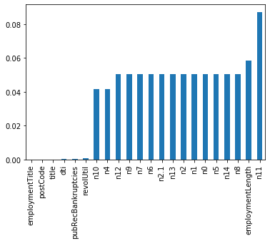
• 纵向了解哪些列存在 “nan”, 并可以把nan的个数打印，主要的目的在于查看某一列nan存在的个数是否真的很大，如果nan存在的过多，说明这一列对label的影响几乎不起作用了，可以考虑删掉。如果缺失值很小一般可以选择填充。
• 另外可以横向比较，如果在数据集中，某些样本数据的大部分列都是缺失的且样本足够的情况下可以考虑删除。

Tips:
比赛大杀器lgb模型可以自动处理缺失值，Task4模型会具体学习模型了解模型哦！

查看训练集测试集中特征属性只有一值的特征

one_value_fea = [col for col in data_train.columns if data_train[col].nunique() <= 1]

one_value_fea_test = [col for col in data_test_a.columns if data_test_a[col].nunique() <= 1]

one_value_fea

['policyCode']

one_value_fea_test

['policyCode']

print(f'There are {len(one_value_fea)} columns in train dataset with one unique value.')
print(f'There are {len(one_value_fea_test)} columns in test dataset with one unique value.')

There are 1 columns in train dataset with one unique value.
There are 1 columns in test dataset with one unique value.

总结：

47列数据中有22列都缺少数据，这在现实世界中很正常。‘policyCode’具有一个唯一值（或全部缺失）。有很多连续变量和一些分类变量。

2.3.5 查看特征的数值类型有哪些，对象类型有哪些

• 特征一般都是由类别型特征和数值型特征组成，而数值型特征又分为连续型和离散型。
• 类别型特征有时具有非数值关系，有时也具有数值关系。比如‘grade’中的等级A，B，C等，是否只是单纯的分类，还是A优于其他要结合业务判断。
• 数值型特征本是可以直接入模的，但往往风控人员要对其做分箱，转化为WOE编码进而做标准评分卡等操作。从模型效果上来看，特征分箱主要是为了降低变量的复杂性，减少变量噪音对模型的影响，提高自变量和因变量的相关度。从而使模型更加稳定。

numerical_fea = list(data_train.select_dtypes(exclude=['object']).columns)
category_fea = list(filter(lambda x: x not in numerical_fea,list(data_train.columns)))

numerical_fea

['id',
 'loanAmnt',
 'term',
 'interestRate',
 'installment',
 'employmentTitle',
 'homeOwnership',
 'annualIncome',
 'verificationStatus',
 'isDefault',
 'purpose',
 'postCode',
 'regionCode',
 'dti',
 'delinquency_2years',
 'ficoRangeLow',
 'ficoRangeHigh',
 'openAcc',
 'pubRec',
 'pubRecBankruptcies',
 'revolBal',
 'revolUtil',
 'totalAcc',
 'initialListStatus',
 'applicationType',
 'title',
 'policyCode',
 'n0',
 'n1',
 'n2',
 'n2.1',
 'n4',
 'n5',
 'n6',
 'n7',
 'n8',
 'n9',
 'n10',
 'n11',
 'n12',
 'n13',
 'n14']

category_fea

['grade', 'subGrade', 'employmentLength', 'issueDate', 'earliesCreditLine']

data_train.grade

0         E
1         D
2         D
3         A
4         C
         ..
799995    C
799996    A
799997    C
799998    A
799999    B
Name: grade, Length: 800000, dtype: object

数值型变量分析，数值型肯定是包括连续型变量和离散型变量的，找出来

• 划分数值型变量中的连续变量和离散型变量

#过滤数值型类别特征
def get_numerical_serial_fea(data,feas):
    numerical_serial_fea = []
    numerical_noserial_fea = []
    for fea in feas:
        temp = data[fea].nunique()
        if temp <= 10:
            numerical_noserial_fea.append(fea)
            continue
        numerical_serial_fea.append(fea)
    return numerical_serial_fea,numerical_noserial_fea
numerical_serial_fea,numerical_noserial_fea = get_numerical_serial_fea(data_train,numerical_fea)

numerical_serial_fea

['id',
 'loanAmnt',
 'interestRate',
 'installment',
 'employmentTitle',
 'annualIncome',
 'purpose',
 'postCode',
 'regionCode',
 'dti',
 'delinquency_2years',
 'ficoRangeLow',
 'ficoRangeHigh',
 'openAcc',
 'pubRec',
 'pubRecBankruptcies',
 'revolBal',
 'revolUtil',
 'totalAcc',
 'title',
 'n0',
 'n1',
 'n2',
 'n2.1',
 'n4',
 'n5',
 'n6',
 'n7',
 'n8',
 'n9',
 'n10',
 'n13',
 'n14']

numerical_noserial_fea

['term',
 'homeOwnership',
 'verificationStatus',
 'isDefault',
 'initialListStatus',
 'applicationType',
 'policyCode',
 'n11',
 'n12']

• 数值类别型变量分析

data_train['term'].value_counts()#离散型变量

3    606902
5    193098
Name: term, dtype: int64

data_train['homeOwnership'].value_counts()#离散型变量

0    395732
1    317660
2     86309
3       185
5        81
4        33
Name: homeOwnership, dtype: int64

data_train['verificationStatus'].value_counts()#离散型变量

1    309810
2    248968
0    241222
Name: verificationStatus, dtype: int64

data_train['initialListStatus'].value_counts()#离散型变量

0    466438
1    333562
Name: initialListStatus, dtype: int64

data_train['applicationType'].value_counts()#离散型变量

0    784586
1     15414
Name: applicationType, dtype: int64

data_train['policyCode'].value_counts()#离散型变量，无用，全部一个值

1.0    800000
Name: policyCode, dtype: int64

data_train['n11'].value_counts()#离散型变量，相差悬殊，用不用再分析

0.0    729682
1.0       540
2.0        24
4.0         1
3.0         1
Name: n11, dtype: int64

data_train['n12'].value_counts()#离散型变量，相差悬殊，用不用再分析

0.0    757315
1.0      2281
2.0       115
3.0        16
4.0         3
Name: n12, dtype: int64

• 数值连续型变量分析

#每个数字特征得分布可视化
f = pd.melt(data_train, value_vars=numerical_serial_fea)
g = sns.FacetGrid(f, col="variable",  col_wrap=2, sharex=False, sharey=False)
g = g.map(sns.distplot, "value")

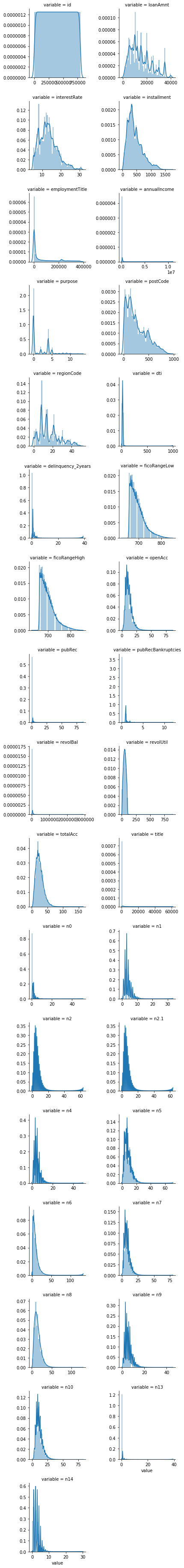
• 查看某一个数值型变量的分布，查看变量是否符合正态分布，如果不符合正太分布的变量可以log化后再观察下是否符合正态分布。
• 如果想统一处理一批数据变标准化 必须把这些之前已经正态化的数据提出
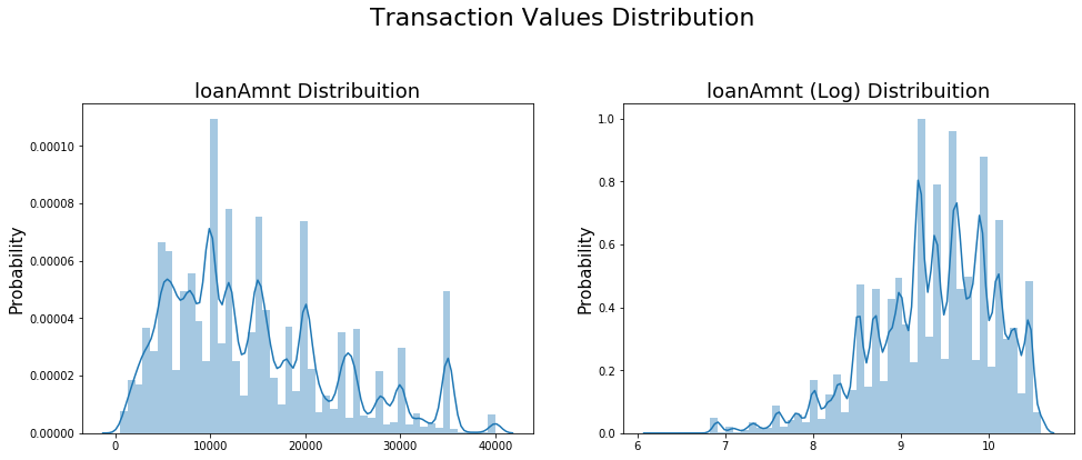
• 正态化的原因：一些情况下正态非正态可以让模型更快的收敛，一些模型要求数据正态（eg. GMM、KNN）,保证数据不要过偏态即可，过于偏态可能会影响模型预测结果。

#Ploting Transaction Amount Values Distribution
plt.figure(figsize=(16,12))
plt.suptitle('Transaction Values Distribution', fontsize=22)
plt.subplot(221)
sub_plot_1 = sns.distplot(data_train['loanAmnt'])
sub_plot_1.set_title("loanAmnt Distribuition", fontsize=18)
sub_plot_1.set_xlabel("")
sub_plot_1.set_ylabel("Probability", fontsize=15)
plt.subplot(222)
sub_plot_2 = sns.distplot(np.log(data_train['loanAmnt']))
sub_plot_2.set_title("loanAmnt (Log) Distribuition", fontsize=18)
sub_plot_2.set_xlabel("")
sub_plot_2.set_ylabel("Probability", fontsize=15)

Text(0, 0.5, 'Probability')

• 非数值类别型变量分析

category_fea

['grade', 'subGrade', 'employmentLength', 'issueDate', 'earliesCreditLine']

data_train['grade'].value_counts()

B    233690
C    227118
A    139661
D    119453
E     55661
F     19053
G      5364
Name: grade, dtype: int64

data_train['subGrade'].value_counts()

C1    50763
B4    49516
B5    48965
B3    48600
C2    47068
C3    44751
C4    44272
B2    44227
B1    42382
C5    40264
A5    38045
A4    30928
D1    30538
D2    26528
A1    25909
D3    23410
A3    22655
A2    22124
D4    21139
D5    17838
E1    14064
E2    12746
E3    10925
E4     9273
E5     8653
F1     5925
F2     4340
F3     3577
F4     2859
F5     2352
G1     1759
G2     1231
G3      978
G4      751
G5      645
Name: subGrade, dtype: int64

data_train['employmentLength'].value_counts()

10+ years    262753
2 years       72358
< 1 year      64237
3 years       64152
1 year        52489
5 years       50102
4 years       47985
6 years       37254
8 years       36192
7 years       35407
9 years       30272
Name: employmentLength, dtype: int64

data_train['issueDate'].value_counts()

2016-03-01    29066
2015-10-01    25525
2015-07-01    24496
2015-12-01    23245
2014-10-01    21461
              ...  
2007-08-01       23
2007-07-01       21
2008-09-01       19
2007-09-01        7
2007-06-01        1
Name: issueDate, Length: 139, dtype: int64

data_train['earliesCreditLine'].value_counts()

Aug-2001    5567
Sep-2003    5403
Aug-2002    5403
Oct-2001    5258
Aug-2000    5246
            ... 
May-1960       1
Apr-1958       1
Feb-1960       1
Aug-1946       1
Mar-1958       1
Name: earliesCreditLine, Length: 720, dtype: int64

data_train['isDefault'].value_counts()

0    640390
1    159610
Name: isDefault, dtype: int64

总结：

• 上面我们用value_counts()等函数看了特征属性的分布，但是图表是概括原始信息最便捷的方式。
• 数无形时少直觉。
• 同一份数据集，在不同的尺度刻画上显示出来的图形反映的规律是不一样的。python将数据转化成图表，但结论是否正确需要由你保证。

2.3.6 变量分布可视化

单一变量分布可视化

plt.figure(figsize=(8, 8))
sns.barplot(data_train["employmentLength"].value_counts(dropna=False)[:20],
            data_train["employmentLength"].value_counts(dropna=False).keys()[:20])
plt.show()

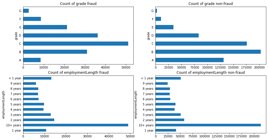
根绝y值不同可视化x某个特征的分布

• 首先查看类别型变量在不同y值上的分布

train_loan_fr = data_train.loc[data_train['isDefault'] == 1]
train_loan_nofr = data_train.loc[data_train['isDefault'] == 0]

fig, ((ax1, ax2), (ax3, ax4)) = plt.subplots(2, 2, figsize=(15, 8))
train_loan_fr.groupby('grade')['grade'].count().plot(kind='barh', ax=ax1, title='Count of grade fraud')
train_loan_nofr.groupby('grade')['grade'].count().plot(kind='barh', ax=ax2, title='Count of grade non-fraud')
train_loan_fr.groupby('employmentLength')['employmentLength'].count().plot(kind='barh', ax=ax3, title='Count of employmentLength fraud')
train_loan_nofr.groupby('employmentLength')['employmentLength'].count().plot(kind='barh', ax=ax4, title='Count of employmentLength non-fraud')
plt.show()

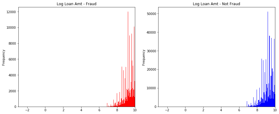
• 其次查看连续型变量在不同y值上的分布

fig, ((ax1, ax2)) = plt.subplots(1, 2, figsize=(15, 6))
data_train.loc[data_train['isDefault'] == 1] \
    ['loanAmnt'].apply(np.log) \
    .plot(kind='hist',
          bins=100,
          title='Log Loan Amt - Fraud',
          color='r',
          xlim=(-3, 10),
         ax= ax1)
data_train.loc[data_train['isDefault'] == 0] \
    ['loanAmnt'].apply(np.log) \
    .plot(kind='hist',
          bins=100,
          title='Log Loan Amt - Not Fraud',
          color='b',
          xlim=(-3, 10),
         ax=ax2)

<matplotlib.axes._subplots.AxesSubplot at 0x126a44b50>

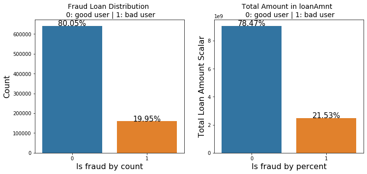
total = len(data_train)
total_amt = data_train.groupby(['isDefault'])['loanAmnt'].sum().sum()
plt.figure(figsize=(12,5))
plt.subplot(121)##1代表行，2代表列，所以一共有2个图，1代表此时绘制第一个图。
plot_tr = sns.countplot(x='isDefault',data=data_train)#data_train‘isDefault’这个特征每种类别的数量**
plot_tr.set_title("Fraud Loan Distribution \n 0: good user | 1: bad user", fontsize=14)
plot_tr.set_xlabel("Is fraud by count", fontsize=16)
plot_tr.set_ylabel('Count', fontsize=16)
for p in plot_tr.patches:
    height = p.get_height()
    plot_tr.text(p.get_x()+p.get_width()/2.,
            height + 3,
            '{:1.2f}%'.format(height/total*100),
            ha="center", fontsize=15) 
percent_amt = (data_train.groupby(['isDefault'])['loanAmnt'].sum())
percent_amt = percent_amt.reset_index()
plt.subplot(122)
plot_tr_2 = sns.barplot(x='isDefault', y='loanAmnt',  dodge=True, data=percent_amt)
plot_tr_2.set_title("Total Amount in loanAmnt  \n 0: good user | 1: bad user", fontsize=14)
plot_tr_2.set_xlabel("Is fraud by percent", fontsize=16)
plot_tr_2.set_ylabel('Total Loan Amount Scalar', fontsize=16)
for p in plot_tr_2.patches:
    height = p.get_height()
    plot_tr_2.text(p.get_x()+p.get_width()/2.,
            height + 3,
            '{:1.2f}%'.format(height/total_amt * 100),
            ha="center", fontsize=15)

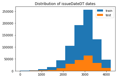
2.3.6 时间格式数据处理及查看

#转化成时间格式  issueDateDT特征表示数据日期离数据集中日期最早的日期（2007-06-01）的天数
data_train['issueDate'] = pd.to_datetime(data_train['issueDate'],format='%Y-%m-%d')
startdate = datetime.datetime.strptime('2007-06-01', '%Y-%m-%d')
data_train['issueDateDT'] = data_train['issueDate'].apply(lambda x: x-startdate).dt.days

#转化成时间格式
data_test_a['issueDate'] = pd.to_datetime(data_train['issueDate'],format='%Y-%m-%d')
startdate = datetime.datetime.strptime('2007-06-01', '%Y-%m-%d')
data_test_a['issueDateDT'] = data_test_a['issueDate'].apply(lambda x: x-startdate).dt.days

plt.hist(data_train['issueDateDT'], label='train');
plt.hist(data_test_a['issueDateDT'], label='test');
plt.legend();
plt.title('Distribution of issueDateDT dates');
#train 和 test issueDateDT 日期有重叠 所以使用基于时间的分割进行验证是不明智的

2.3.7 掌握透视图可以让我们更好的了解数据

#透视图 索引可以有多个，“columns（列）”是可选的，聚合函数aggfunc最后是被应用到了变量“values”中你所列举的项目上。
pivot = pd.pivot_table(data_train, index=['grade'], columns=['issueDateDT'], values=['loanAmnt'], aggfunc=np.sum)

pivot

2.3.8 用pandas_profiling生成数据报告

import pandas_profiling

pfr = pandas_profiling.ProfileReport(data_train)
pfr.to_file("./example.html")

2.4 总结

数据探索性分析是我们初步了解数据，熟悉数据为特征工程做准备的阶段，甚至很多时候EDA阶段提取出来的特征可以直接当作规则来用。可见EDA的重要性，这个阶段的主要工作还是借助于各个简单的统计量来对数据整体的了解，分析各个类型变量相互之间的关系，以及用合适的图形可视化出来直观观察。希望本节内容能给初学者带来帮助，更期待各位学习者对其中的不足提出建议。

END.
【 言溪：Datawhale成员，金融风控爱好者。知乎地址：https://www.zhihu.com/people/exuding】

关于Datawhale：
Datawhale是一个专注于数据科学与AI领域的开源组织，汇集了众多领域院校和知名企业的优秀学习者，聚合了一群有开源精神和探索精神的团队成员。Datawhale 以“for the learner，和学习者一起成长”为愿景，鼓励真实地展现自我、开放包容、互信互助、敢于试错和勇于担当。同时 Datawhale 用开源的理念去探索开源内容、开源学习和开源方案，赋能人才培养，助力人才成长，建立起人与人，人与知识，人与企业和人与未来的联结。
本次数据挖掘路径学习，专题知识将在天池分享，详情可关注Datawhale：