GCN
参考:
[Github源码] tkipf/pygcn: Graph Convolutional Networks in PyTorch (github.com)
理论-supplement
1.半监督学习是什么?体现在哪里?
有监督分类:是从已有数据集%7D#card=math&code=%7B%28x_n%2Cy_n%29%7D&id=V8VI8),
中学习一个函数
#card=math&code=y%3Df%28x%29&id=JKT52),其中
是数据特征,
是数据的类别标签,数据集样本总数是
。
无监督聚类:已知数据集,
,标签信息
未知,需要将相似的样本聚到一类中。
半监督聚类:一般假设数据集中有个样本的标签已知,而
个样本的标签未知,即
,
和
,
。
2.如何得到每个节点的embedding?
个人理解:model部分,logsoftmax前的x就是每个节点的embedding
def forward(self, x, adj):x = F.relu(self.gc1(x, adj)) # adj即公式Z=softmax(A~Relu(A~XW(0))W(1))中的A~x = F.dropout(x, self.dropout, training=self.training) # x要dropoutx = self.gc2(x, adj) #embeddingreturn F.log_softmax(x, dim=1)
3. 网络结构(核心)
由论文可知,代码的核心公式:
%3Dsoftmax(%5Chat%20A%20ReLU(%5Chat%20AXW%5E%7B(0)%7D)W%5E%7B(1)%7D)%0A#card=math&code=Z%3Df%28X%2CA%29%3Dsoftmax%28%5Chat%20A%20ReLU%28%5Chat%20AXW%5E%7B%280%29%7D%29W%5E%7B%281%29%7D%29%0A&id=g4cJW)
其中:


实现了两层网络
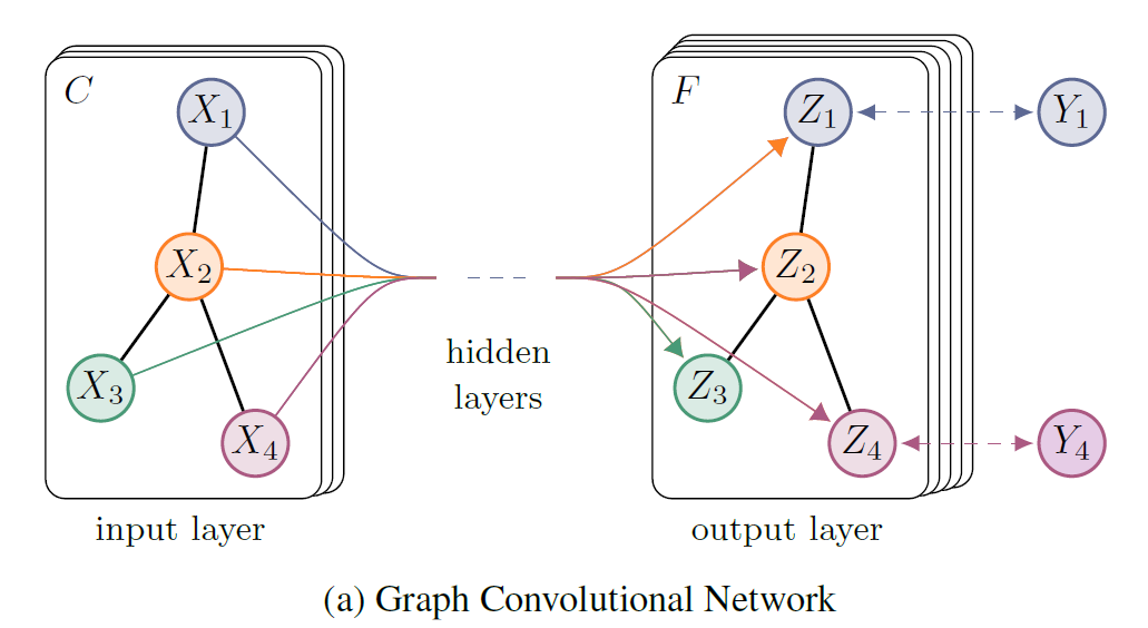
- 隐层的faeture maps的数量为H,输入层数量为C,输出层为F
- 权重
%7D%5Cin%20%5Cmathbb%20R%5E%7BC%5Ctimes%20H%7D#card=math&code=W%5E%7B%280%29%7D%5Cin%20%5Cmathbb%20R%5E%7BC%5Ctimes%20H%7D&id=ScbsR)为输入层到隐层的权值矩阵
- 权重
%7D%5Cin%20%5Cmathbb%20R%5E%7BH%5Ctimes%20F%7D#card=math&code=W%5E%7B%281%29%7D%5Cin%20%5Cmathbb%20R%5E%7BH%5Ctimes%20F%7D&id=AYb7X)为隐层到输出层的权值矩阵
setup.py
一、构建工具setup.py的应用场景
在安装python的相关模块和库时,我们一般使用“pip install 模块名”或者“python setup.py install”,前者是在线安装,会安装该包的相关依赖包;后者是下载源码包然后在本地安装,不会安装该包的相关依赖包。
在编写相关系统时,python 如何实现连同依赖包一起打包发布?
假如我在本机开发一个程序,需要用到python的redis、mysql模块以及自己编写的redis_run.py模块。我怎么实现在服务器上去发布该系统,如何实现依赖模块和自己编写的模块redis_run.py一起打包,实现一键安装呢?同时将自己编写的redis_run.py模块以exe文件格式安装到python的全局执行路径C:\Python27\Scripts下呢?这时就需要setup进行实现。
使用python的构建工具setup.py了,使用此构建工具可以实现上述应用场景需求,只需在 setup.py 文件中写明依赖的库和版本,然后到目标机器上使用python setup.py install安装。
二、setup.py介绍
#!/usr/bin/env python
# coding=utf-8

from setuptools import setup

'''
把redis服务打包成C:\Python27\Scripts下的exe文件
'''

setup(
    name="RedisRun",  #pypi中的名称,pip或者easy_install安装时使用的名称,或生成egg文件的名称
    version="1.0",
    author="Andreas Schroeder",
    author_email="andreas@drqueue.org",
    description=("This is a service of redis subscripe"),
    license="GPLv3",
    keywords="redis subscripe",
    url="https://ssl.xxx.org/redmine/projects/RedisRun",
    packages=['RedisRun'],  # 需要打包的目录列表

    # 需要安装的依赖
    install_requires=[
        'redis>=2.10.5',
        'setuptools>=16.0',
    ],

    # 添加这个选项,在windows下Python目录的scripts下生成exe文件
    # 注意:模块与函数之间是冒号:
    entry_points={'console_scripts': [
        'redis_run = RedisRun.redis_run:main',
    ]},

    # long_description=read('README.md'),
    classifiers=[  # 程序的所属分类列表
        "Development Status :: 3 - Alpha",
        "Topic :: Utilities",
        "License :: OSI Approved :: GNU General Public License (GPL)",
    ],
    # 此项需要,否则卸载时报windows error
    zip_safe=False
)
—name 包名称
—version (-V) 包版本
—author 程序的作者
—author_email 程序的作者的邮箱地址
—maintainer 维护者
—maintainer_email 维护者的邮箱地址
—url 程序的官网地址
—license 程序的授权信息
—description 程序的简单描述
—long_description 程序的详细描述
—platforms 程序适用的软件平台列表
—classifiers 程序的所属分类列表
—keywords 程序的关键字列表
—packages 需要处理的包目录(包含init.py的文件夹)
—py_modules 需要打包的python文件列表
—download_url 程序的下载地址
—cmdclass
—data_files 打包时需要打包的数据文件,如图片,配置文件等
—scripts 安装时需要执行的脚步列表
—package_dir 告诉setuptools哪些目录下的文件被映射到哪个源码包。一个例子:package_dir = {‘’: ‘lib’},表示“root package”中的模块都在lib 目录中。
—requires 定义依赖哪些模块
—provides定义可以为哪些模块提供依赖
—find_packages() 对于简单工程来说,手动增加packages参数很容易,刚刚我们用到了这个函数,它默认在和setup.py同一目录下搜索各个含有 init.py的包。
其实我们可以将包统一放在一个src目录中,另外,这个包内可能还有aaa.txt文件和data数据文件夹。另外,也可以排除一些特定的包
find_packages(exclude=["*.tests", "*.tests.*", "tests.*", "tests"])
—install_requires = [“requests”] 需要安装的依赖包
—entry_points 动态发现服务和插件,下面详细讲
init.py
__init__.py 的作用是让一个呈结构化分布(以文件夹形式组织)的代码文件夹变成可以被导入import的软件包。
实际上,如果目录中包含了 __init__.py 时,当用 import 导入该目录时,会执行__init__.py 里面的代码。
from __future__ import print_function  # 导入py3的输出函数,使得py2也可以用
from __future__ import division  # 导入division,'/'表示精确除法 '//'表示整除

from .layers import *
from .models import *
from .utils import *
__future__
from future import absolute_import的作用
这是相对引用和绝对引用的概念,从相对导入变成绝对导入,大概意指你每次用import X时候都是在sys.path(即python的搜索模块的路径集)里面找X包,这个其实不需要深究,只要知道py3的import用法,加上这句话py2时候也能按照py3的import语法去正常使用。
from future import division的作用
division(精确除法),当我们没有在程序中导入该特征时,”/“操作符执行的是截断除法(Truncating Division),当我们导入精确除法之后,”/“执行的是精确除法,如下所示:
>>> 3/4
0
>>> from __future__ import division
>>> 3/4
0.75
导入精确除法后,若要执行截断除法,可以使用”//“操作符:
>>> 3//4
0
from future import print_function的作用
超前使用python3的print函数。
举例如下:
在python2.x的环境是使用下面语句,则第二句语法检查通过,第三句语法检查失败
from __future__ import print_function
print('you are good')
print 'you are good'
utils.py
def encode_onehot(labels)
'''
先将所有由字符串表示的标签数组用set保存,set的重要特征就是元素没有重复,
因此表示成set后可以直接得到所有标签的总数,随后为每个标签分配一个编号,创建一个单位矩阵,
单位矩阵的每一行对应一个one-hot向量,也就是np.identity(len(classes))[i, :],
再将每个数据对应的标签表示成的one-hot向量,类型为numpy数组
'''
def encode_onehot(labels):
    # set() Build an unordered collection of unique elements.
    # 将labels转为(无重复数据)无序集合set
    classes = set(labels)
    # enumerate函数返回enumerate枚举类型,用于将一个可遍历的数据对象组合为一个索引序列
    # enumerate(classes)返回(0, classes[0]), (1, classes[1]), (2, classes[2]), ...
    # np.identity创建标识矩阵 标识数组是单位矩阵(对角线值为1)。
    # classes_dict是一个key为labels的值,value为矩阵一行的字典
    classes_dict = {c: np.identity(len(classes))[i, :] for i, c in
                    enumerate(classes)}
    # map(function,*iterables) 即将iterables中元素依次作为funcation的输入
    # labels_onehot是输入的labels按照classes_dict中的对应关系进行onehot之后的输出
    labels_onehot = np.array(list(map(classes_dict.get, labels)),
                             dtype=np.int32)
    return labels_onehot
def load_data(path=”../data/cora/“, dataset=”cora”)
def load_data(path="../data/cora/", dataset="cora"):
    """加载数据 Load citation network dataset (cora only for now)"""
    print('Loading {} dataset...'.format(dataset))

    # np.genfromtxt(file_name,dtype,...)读取text文件 genfromtxt运行两个主循环。
    # 第一个循环以字符串序列转换文件的每一行。第二个循环将(按照delimiter划分行得到的字符串(默认情况下,
    # 任何连续的空格充当分隔符))每个字符串转换为适当的数据类型。这种机制比单循环慢,但具有更大的灵活性。
    idx_features_labels = np.genfromtxt("{}{}.content".format(path, dataset),
                                        dtype=np.dtype(str))
    # sp.csr_matrix对数据进行压缩处理
    features = sp.csr_matrix(idx_features_labels[:, 1:-1], dtype=np.float32)
    labels = encode_onehot(idx_features_labels[:, -1])
    # 这里的label为onthot格式,如第一类代表[1,0,0,0,0,0,0]
    # content file的每一行的格式为 : <paper_id> <word_attributes>+ <class_label>
    #    分别对应 0, 1:-1, -1
    # feature为第二列到倒数第二列,labels为最后一列

    # build graph
    idx = np.array(idx_features_labels[:, 0], dtype=np.int32)
    # 由于文件中节点并非是按顺序排列的,因此建立一个编号为0-(node_size-1)的哈希表idx_map,
    # idx_map哈希表中每一项为id: number,即节点id对应的编号为number
    idx_map = {j: i for i, j in enumerate(idx)}
    # cites file的每一行格式为:  <cited paper ID>  <citing paper ID>
    # edges_unordered为直接从边表文件中直接读取的结果,是一个(edge_num, 2)的数组,每一行表示一条边两个端点的idx (被引用论文,引用论文)
    edges_unordered = np.genfromtxt("{}{}.cites".format(path, dataset),
                                    dtype=np.int32)
    # 边的edges_unordered中存储的是端点id,要将每一项的id换成编号。
    # 在idx_map中以idx作为键查找得到对应节点的编号,reshape成与edges_unordered形状一样的数组
    edges = np.array(list(map(idx_map.get, edges_unordered.flatten())),
                     dtype=np.int32).reshape(edges_unordered.shape)
    # 获得邻接矩阵
    # sp.coo_matrix((data,(row,col)),shape) 返回一个压缩后的matrix
    # 根据coo矩阵性质,这一段的作用就是,网络有多少条边,邻接矩阵就有多少个1,
    # 所以先创建一个长度为edge_num的全1数组,每个1的填充位置就是一条边中两个端点的编号,
    # 即edges[:, 0], edges[:, 1],矩阵的形状为(node_size, node_size)
    adj = sp.coo_matrix((np.ones(edges.shape[0]), (edges[:, 0], edges[:, 1])),
                        shape=(labels.shape[0], labels.shape[0]),  # labels.shape[0]代表了有多少节点
                        dtype=np.float32)

    # build symmetric adjacency matrix
    # 注意由于edges中边是单向的,所有构建的adj矩阵也是有向图邻接矩阵  所以需要转换成无向图邻接矩阵
    adj = adj + adj.T.multiply(adj.T > adj) - adj.multiply(adj.T > adj)
    # TODO 疑问:为什么对feature进行规范化?
    features = normalize(features)
    adj = normalize(adj + sp.eye(adj.shape[0]))
    # adj + sp.eye(adj.shape[0])对应公式:\tilde A = A + I
    # normalize(\tilde A)对应公式:\tilde D^{-1/2} \tilde A \tilde D^{-1/2}
    # TODO 疑问:为什么normalize(\tilde A)对应 \tilde D^{-1/2} \tilde A \tilde D^{-1/2}

    # 分别构建训练集、验证集、测试集的范围
    idx_train = range(140)
    idx_val = range(200, 500)
    idx_test = range(500, 1500)

    # features.todense()作用是将稀疏矩阵转为稠密矩阵(即将压缩的矩阵转为未压缩的矩阵) 类型是matrix
    features = torch.FloatTensor(np.array(features.todense()))
    # np.where(condition)只提供condition时,作用相当于np.asarray(condition).nonzero()
    # 即Return the indices of unmasked elements that are not zero.
    # 这里的坐标以tuple的形式给出,通常原数组有多少维,输出的tuple中就包含几个数组,分别对应符合条件元素的各维坐标。
    labels = torch.LongTensor(np.where(labels)[1])  # np.where(labels)[1]取labels中非零的列索引(即第二维)构成一维元组
    # 此时labels变为一维的LongTensor  每个元素为对应<class_label>在onehot后的索引

    # 邻接矩阵转为tensor处理
    adj = sparse_mx_to_torch_sparse_tensor(adj)

    idx_train = torch.LongTensor(idx_train)
    idx_val = torch.LongTensor(idx_val)
    idx_test = torch.LongTensor(idx_test)

    return adj, features, labels, idx_train, idx_val, idx_test
np.where
>>> labels
tensor([[1, 0, 2],
        [0, 1, 1],
        [0, 2, 1]], dtype=torch.int32)
>>> np.where(labels)
(array([0, 0, 1, 1, 2, 2], dtype=int64), array([0, 2, 1, 2, 1, 2], dtype=int64))
>>> np.where(labels)[1]  # 输出每个大于1的元素的列数构成的数组
array([0, 2, 1, 2, 1, 2], dtype=int64)
疑问
TODO 疑问:为什么对feature进行规范化?
features = normalize(features)
TODO 疑问:为什么normalize(\tilde A)对应 \tilde D^{-1/2} \tilde A \tilde D^{-1/2}
adj = normalize(adj + sp.eye(adj.shape[0]))
# adj + sp.eye(adj.shape[0])对应公式:\tilde A = A + I
# normalize(\tilde A)对应公式:\tilde D^{-1/2} \tilde A \tilde D^{-1/2}
代码中实现的好像是:
def normalize(mx)
def normalize(mx):
    """
    Row-normalize sparse matrix
    将矩阵进行行规范化,即每个元素除以这一行的和
    """
    rowsum = np.array(mx.sum(1))  # 求每行和
    r_inv = np.power(rowsum, -1).flatten()  # 获得每行和对应倒数构成的一维np数组
    r_inv[np.isinf(r_inv)] = 0.  # 将分母为零(即行和为0)的数据设为0
    r_mat_inv = sp.diags(r_inv)  # 以r_inv为对角线上数据绘制对角矩阵
    mx = r_mat_inv.dot(mx)  # 对输入矩阵进行按行规范化
    return mx
关于axis的理解
1. axis的参数的取值
有两维的数组,每一维又拥有三个数组,这个数组里面拥有四个元素,即a[2][3][4]。如果我们要将这个a数组中的第一个元素1定位出来,则我们会输入a[0][0][0]。而这个axis的取值就是这个精确定位某个元素需要经过多少数组的长度,在这里是3,所以axis的取值有0,1,2。如果一个数组精确到某个元素需要a[n0][n1][n2][…][n],则axis的取值就是n。
2. 理解参数axis取值对sum结果的影响
axis的取值0,1,2。在这里,精确定位到某个元素可以用a[n0][n1][n2]表示。n0的取值是0,1(数组两维),代表第一个索引;n1的取值是0,1,2(每一维数组拥有3个子数组),代表第二个索引;n2的取值是0,1,2,3(每个子数组有4个元素),代表第三个索引,这几个取值在后面会用到。
如果axis = 0:
axis=0,对应n0已经确定下来,即n0取值定为0,1。所以sum每个元素的求和公式是。接下来确定sum的行数和列数,n1的取值是0,1,2,为3个数,代表行数,n2的取值是0,1,2,3,为4个数,代表列数,所以sum为3*4的数组。
如果axis = 1:
axis=1,对应n1已经确定下来,即n1取值定为0,1,2。所以sum每个元素的求和公式是。接下来确定sum的行数和列数,n0的取值是0,1,为2个数,代表行数,n2的取值是0,1,2,3,为4个数,代表列数,所以sum为2*4的数组。
……
def accuracy(output, labels)
def accuracy(output, labels):
    """
    输出预测准确率
    """
    # output是tensor格式 output.max(1)[1]将返回概率最大的标签的下标值
    preds = output.max(1)[1].type_as(labels)  # 使用type_as(tesnor)将张量转换为给定类型的张量。
    # preds等于labels中对应值的返回true,否则返回false    .double()将true转为1.,false转为0.
    correct = preds.eq(labels).double()
    correct = correct.sum()
    return correct / len(labels)
tensor.max
>>> c
tensor([[ 0,  0,  0,  2,  5,  0,  0],
        [ 0,  0,  0,  6,  0,  7,  0],
        [ 0,  0,  0,  0, 10,  0,  0],
        [ 0,  0,  0,  0,  0,  0,  0],
        [ 0,  0,  0,  0,  0,  0,  0],
        [ 0,  0,  0,  0,  0,  0,  0],
        [ 0,  0,  0,  0,  0,  0,  0]], dtype=torch.int32)
>>> torch.IntTensor(c).max(1)
torch.return_types.max(
values=tensor([ 5,  7, 10,  0,  0,  0,  0], dtype=torch.int32),
indices=tensor([4, 5, 4, 0, 0, 0, 0]))
>>> torch.IntTensor(c).max(1)[1] # 返回的是取最大值的下标
tensor([4, 5, 4, 0, 0, 0, 0])
def sparse_mx_to_torch_sparse_tensor(sparse_mx)
def sparse_mx_to_torch_sparse_tensor(sparse_mx):
    """Convert a scipy sparse matrix to a torch sparse tensor.把一个sparse matrix转为torch中的稀疏张量"""
    # tocoo()作用Convert this matrix to COOrdinate format
    sparse_mx = sparse_mx.tocoo().astype(np.float32)
    indices = torch.from_numpy(
        np.vstack((sparse_mx.row, sparse_mx.col)).astype(np.int64))  # np.vstack(a,b)将a和b按行堆叠
    values = torch.from_numpy(sparse_mx.data)  # numpy中的ndarray转化成pytorch中的tensor : torch.from_numpy()
    shape = torch.Size(sparse_mx.shape)
    return torch.sparse.FloatTensor(indices, values, shape)
疑问:torch.sparse.FloatTensor()好像有问题?
numpy中的ndarray转化成pytorch中的tensor : torch.from_numpy()
pytorch中的tensor转化成numpy中的ndarray : tensor.numpy()
layer.py
import math

import torch

from torch.nn.parameter import Parameter
from torch.nn.modules.module import Module


class GraphConvolution(Module):
    """
    Simple GCN layer, similar to https://arxiv.org/abs/1609.02907
    """

    def __init__(self, in_features, out_features, bias=True):
        """
        in_features:该层输入单元数
        out_features:该层输出单元数
        bias:是否有偏置
        """
        super(GraphConvolution, self).__init__()
        self.in_features = in_features
        self.out_features = out_features
        # 常见用法self.v = torch.nn.Parameter(torch.FloatTensor(hidden_size)):
        # 首先可以把这个函数理解为类型转换函数,将一个不可训练的类型Tensor转换成可以训练的类型parameter并将这个parameter
        # 绑定到这个module里面,所以经过类型转换这个self.v变成了模型的一部分,成为了模型中根据训练可以改动的参数了。
        # 使用这个函数的目的也是想让某些变量在学习的过程中不断的修改其值以达到最优化。
        self.weight = Parameter(torch.FloatTensor(in_features, out_features))
        # self.weight是in_features*out_features的矩阵
        if bias:
            self.bias = Parameter(torch.FloatTensor(out_features))
        else:
            # Parameters与register_parameter都会向parameters写入参数,但是后者可以支持字符串命名
            self.register_parameter('bias', None)
        self.reset_parameters()

    def reset_parameters(self):
        """初始化参数  重置参数为随机数"""
        # stdv设为 1/out_features  即输出单元数分之一
        stdv = 1. / math.sqrt(self.weight.size(1))
        # uniform_(b,e)生成[b,e)范围内的数,tensor.uniform_作用:将tensor用从均匀分布中抽样得到的值填充。
        self.weight.data.uniform_(-stdv, stdv)
        if self.bias is not None:
            self.bias.data.uniform_(-stdv, stdv)

    def forward(self, input, adj):
        """
        前馈运算 即计算 \hat A input W   其中 \hat A= \tilde D^{-1/2} \tilde A \tilde D^{-1/2}
        """
        # torch.mm(a, b)是矩阵a和b矩阵相乘
        # torch.mul(a, b)是矩阵a和b对应位相乘
        support = torch.mm(input, self.weight)
        # input维度:样本数m*输入特征数in_features  weight维度:输入特征数in_features*输出特征数out_features
        # support维度:样本数m*输出特征数out_features
        output = torch.spmm(adj, support)  # torch.spmm(a,b) 稀疏矩阵相乘
        # 加上偏执bias
        if self.bias is not None:
            return output + self.bias
        else:
            return output

    def __repr__(self):
        """
        print(该对象)时调用__repr__  返回值必须是字符串类型
        repr能把一个对象用字符串的形式表达出来以便辨认,这就是“字符串表示形式”。
        """
        return self.__class__.__name__ + ' (' \
               + str(self.in_features) + ' -> ' \
               + str(self.out_features) + ')'
疑问:为什么层layer与模型model都继承于nn.Module
models.py
import torch.nn as nn
import torch.nn.functional as F
from pygcn.layers import GraphConvolution


class GCN(nn.Module):
    def __init__(self, nfeat, nhid, nclass, dropout):
        """
        nfeat:输入层单元数即特征feature的维度
        nhid:隐藏层的隐藏单元
        nclass:输出层单元数即分类的类别数
        dropout:dropout的概率值
        """
        super(GCN, self).__init__()

        self.gc1 = GraphConvolution(nfeat, nhid)  # gc1输入尺寸nfeat,输出尺寸nhid
        self.gc2 = GraphConvolution(nhid, nclass)  # gc2输入尺寸nhid,输出尺寸ncalss
        self.dropout = dropout

    def forward(self, x, adj):
        """
        输入分别是特征和邻接矩阵。最后输出为输出层做log_softmax变换的结果
        对应公式:Z=softmax(\hat A Relu(\hat A X W(0)) W(1))
        """
        # torch.nn.functional 其中是一些常用的relu、dropout的函数形式实现
        x = F.relu(self.gc1(x, adj))  # self.gc1(x, adj)调用GraphConvolution的forward(input, adj)函数
        x = F.dropout(x, self.dropout, training=self.training)  # 进行dropout
        x = self.gc2(x, adj)  # adj即公式Z=softmax(\hat A Relu(\hat A X W(0)) W(1))中的\hat A
        return F.log_softmax(x, dim=1)
train.py
from __future__ import division
from __future__ import print_function

import time
import argparse  # argparse 是python自带的命令行参数解析包,可以用来方便地读取命令行参数
import numpy as np

import torch
import torch.nn.functional as F
import torch.optim as optim

from pygcn.utils import load_data, accuracy
from pygcn.models import GCN

# Training settings
parser = argparse.ArgumentParser()
parser.add_argument('--no-cuda', action='store_true', default=False,
                    help='Disables CUDA training.')
parser.add_argument('--fastmode', action='store_true', default=False,
                    help='Validate during training pass.')  # Validate验证
parser.add_argument('--seed', type=int, default=42, help='Random seed.')
parser.add_argument('--epochs', type=int, default=200,
                    help='Number of epochs to train.')
parser.add_argument('--lr', type=float, default=0.01,
                    help='Initial learning rate.')
parser.add_argument('--weight_decay', type=float, default=5e-4,
                    help='Weight decay (L2 loss on parameters).')
parser.add_argument('--hidden', type=int, default=16,
                    help='Number of hidden units.')
parser.add_argument('--dropout', type=float, default=0.5,
                    help='Dropout rate (1 - keep probability).')

args = parser.parse_args()
# not args.no_cuda 表示不禁用cuda    torch.cuda.is_available()本机cuda可用
args.cuda = not args.no_cuda and torch.cuda.is_available()

np.random.seed(args.seed)  # 随机数种子
torch.manual_seed(args.seed)  # 对torch.rand(1,2)设置CPU随机数种子
# TODO 疑问:这个np设置的种子和torch.manual_seed设置的种子,对于torch.Tensor(r,c).uniform_(f,t)有用吗

if args.cuda:  # 设置GPU随机数种子
    torch.cuda.manual_seed(args.seed)

# Load data
adj, features, labels, idx_train, idx_val, idx_test = load_data()

# Model and optimizer
model = GCN(nfeat=features.shape[1],
            nhid=args.hidden,
            nclass=labels.max().item() + 1,  # 加一是因为labels的下标是从0开始的
            dropout=args.dropout)
optimizer = optim.Adam(model.parameters(),
                       lr=args.lr, weight_decay=args.weight_decay)

# 数据写入cuda,便于后续加速
if args.cuda:
    model.cuda()  # .cuda()会分配到显存里(如果gpu可用)
    features = features.cuda()
    adj = adj.cuda()
    labels = labels.cuda()
    idx_train = idx_train.cuda()
    idx_val = idx_val.cuda()
    idx_test = idx_test.cuda()


def train(epoch):
    """
    训练函数(一次函数是一轮)
    """
    t = time.time()  # 返回当前时间
    model.train()  # TODO  这里是做什么?
    # pytorch中每一轮batch需要设置optimizer.zero_gra
    optimizer.zero_grad()  # optimizer.zero_grad()意思是把梯度置零,也就是把loss关于weight的导数变成0.
    output = model(features, adj)  # 获得输出
    # 由于在算output时已经使用了log_softmax(log_softmax()相当于先求softmax再求log),这里使用的损失函数就是NLLloss,
    # 如果前面没有加log运算,这里就要使用CrossEntropyLoss了
    # 损失函数NLLLoss() 的输入是一个对数概率向量和一个目标标签. 它不会为我们计算对数概率,
    # 适合最后一层是log_softmax()的网络. 损失函数 CrossEntropyLoss() 与 NLLLoss() 类似,
    # 唯一的不同是它为我们去做 softmax.可以理解为:CrossEntropyLoss()=log_softmax() + NLLLoss()
    # NLLloss 负对数似然损失
    loss_train = F.nll_loss(output[idx_train], labels[idx_train])
    acc_train = accuracy(output[idx_train], labels[idx_train])  # 计算准确率
    loss_train.backward()  # 反向求导  Back Propagation
    optimizer.step()  # 更新所有的参数  Gradient Descent

    if not args.fastmode:
        # Evaluate validation set performance separately,
        # deactivates dropout during validation run.
        model.eval()  # eval()函数用来执行一个字符串表达式,并返回表达式的值
        output = model(features, adj)

    loss_val = F.nll_loss(output[idx_val], labels[idx_val])  # 验证集的损失函数
    acc_val = accuracy(output[idx_val], labels[idx_val])
    print('Epoch: {:04d}'.format(epoch+1),
          'loss_train: {:.4f}'.format(loss_train.item()),
          'acc_train: {:.4f}'.format(acc_train.item()),
          'loss_val: {:.4f}'.format(loss_val.item()),
          'acc_val: {:.4f}'.format(acc_val.item()),
          'time: {:.4f}s'.format(time.time() - t))


# 定义测试函数,相当于对已有的模型在测试集上运行对应的loss与accuracy
def test():
    model.eval()
    output = model(features, adj)
    loss_test = F.nll_loss(output[idx_test], labels[idx_test])
    acc_test = accuracy(output[idx_test], labels[idx_test])
    print("Test set results:",
          "loss= {:.4f}".format(loss_test.item()),
          "accuracy= {:.4f}".format(acc_test.item()))


# Train model
t_total = time.time()
# 逐个epoch进行train
for epoch in range(args.epochs):
    train(epoch)
print("Optimization Finished!")
print("Total time elapsed: {:.4f}s".format(time.time() - t_total))

# Testing
test()
loss函数之NLLLoss,CrossEntropyLoss
假设已有input: Tensor(mn矩阵,每行是一个样本的预测对应分类的概率(共n个分类)),已有target: Tensor(1m矩阵,每个数代表对应样本的实际分类下标)
torch.nn.functional.softmax(input)
对应公式softmax:
%3D%5Cfrac%7Bexp(x_i)%7D%7B%5Csum_j%20exp(x_j)%7D%0A#card=math&code=Softmax%28x_i%29%3D%5Cfrac%7Bexp%28x_i%29%7D%7B%5Csum_j%20exp%28x_j%29%7D%0A&id=zUBY0)
torch.nn.functional.log_softmax(input)
对应公式softmax取了个log:
%3D%5Clog(%5Cfrac%7B%5Cexp(x_i)%7D%7B%5Csum_j%5Cexp(x_j)%7D)%0A#card=math&code=LogSoftmax%28x_i%29%3D%5Clog%28%5Cfrac%7B%5Cexp%28x_i%29%7D%7B%5Csum_j%5Cexp%28x_j%29%7D%29%0A&id=EaZ9Q)
torch.nn.functional.nll_loss(input, target)
负对数似然损失函数(The negative log likelihood loss.),用于处理多分类问题,输入是对数化的概率值(即torch.nn.functional.log_softmax的输出)。
%3D%0A%5Cbegin%7Bcases%7D%0A%5Csum%7Bn%3D1%7D%5E%7BN%7D%5Cfrac%7B1%7D%7B%5Csum%7Bn%3D1%7D%5E%7BN%7Dw%7By_n%7D%7Dl_n%2C%20%5Cquad%20if%5C%3A%5C%3Areducation%3D’mean’%3B%5C%5C%0A%5Csum%7Bn%3D1%7D%5E%7BN%7Dln%2C%5Cquad%20if%5C%3A%5C%3Areducation%3D’sum’.%0A%5Cend%7Bcases%7D%0A#card=math&code=%5Cmathscr%7Bl%7D%28x%2Cy%29%3D%0A%5Cbegin%7Bcases%7D%0A%5Csum%7Bn%3D1%7D%5E%7BN%7D%5Cfrac%7B1%7D%7B%5Csum%7Bn%3D1%7D%5E%7BN%7Dw%7Byn%7D%7Dl_n%2C%20%5Cquad%20if%5C%3A%5C%3Areducation%3D%27mean%27%3B%5C%5C%0A%5Csum%7Bn%3D1%7D%5E%7BN%7Dl_n%2C%5Cquad%20if%5C%3A%5C%3Areducation%3D%27sum%27.%0A%5Cend%7Bcases%7D%0A&id=XGnrR)
torch.nn.functional.nll_loss实际就是取出input中依此对应target位置的值,然后每个前加负号,再求平均或求和(reducation决定)。
torch.nn.functional.cross_entropy(input, target)
交叉熵,相当于log_softmax+nll_loss,对应表达式:
%3D-%5Clog(%5Cfrac%7B%5Cexp(x%5Bclass%5D)%7D%7B%5Csum_j%5Cexp(x%5Bj%5D)%7D)%5C%5C%3D-x%5Bclass%5D%2B%5Clog(%5Csum_j%5Cexp(x%5Bj%5D))%0A#card=math&code=loss%28x%2Cclass%29%3D-%5Clog%28%5Cfrac%7B%5Cexp%28x%5Bclass%5D%29%7D%7B%5Csum_j%5Cexp%28x%5Bj%5D%29%7D%29%5C%5C%3D-x%5Bclass%5D%2B%5Clog%28%5Csum_j%5Cexp%28x%5Bj%5D%29%29%0A&id=NSCjT)
对应实际交叉熵公式:
%3D-%5Csum%20y*%5Clog%20x%0A%3D%5Cbegin%7Bcases%7D%0A-%5Clog%20x%2Cy%3D1%5C%5C%0A0%2Cy%3D0%0A%5Cend%7Bcases%7D%0A#card=math&code=l%28x%2Cy%29%3D-%5Csum%20y%2A%5Clog%20x%0A%3D%5Cbegin%7Bcases%7D%0A-%5Clog%20x%2Cy%3D1%5C%5C%0A0%2Cy%3D0%0A%5Cend%7Bcases%7D%0A&id=DB1rW)
其中y是label,x是预测prediction的结果,所以其实交叉熵损失就是负的target对应位置的输出结果x再取-log。这个计算过程刚好就是log_softmax()再进行nll_loss()。
torch.nn.functional.binary_cross_entropy(input,target)
BCELoss(Binary Cross Entropy Loss ),就是交叉熵应用于二分类时候的特殊形式,一般都和sigmoid一起用,表达式就是二分类交叉熵:
*log(1-x_n)%5D%5D%0A#card=math&code=l_n%3D-w_n%5By_n%2A%5Clog%20x_n%2B%281-y_n%29%2Alog%281-x_n%29%5D%5D%0A&id=Q75V4)
和多分类交叉熵的区别在于:不仅考虑了的样本,也考虑了
的样本的损失。
疑问
疑问:这个np设置的种子和torch.manualseed设置的种子,对于torch.Tensor(r,c).uniform(f,t)有用吗
np.random.seed(args.seed) # 随机数种子
torch.manual_seed(args.seed) # 对torch.rand(1,2)设置CPU随机数种子

若有收获,就点个赞吧
0 人点赞
