相关性系数

  计算两个数据集的相关性是统计中的常用操作。在MLlib中提供了计算多个数据集两两相关的方法。目前支持的相关性方法有皮尔森(Pearson)相关和斯皮尔曼(Spearman)相关。

  Statistics提供方法计算数据集的相关性。根据输入的类型，两个RDD[Double]或者一个RDD[Vector]，输出将会是一个Double值或者相关性矩阵。下面是一个应用的例子。

import org.apache.spark.SparkContext
import org.apache.spark.mllib.linalg._
import org.apache.spark.mllib.stat.Statistics
val sc: SparkContext = ...
val seriesX: RDD[Double] = ... // a series
val seriesY: RDD[Double] = ... // must have the same number of partitions and cardinality as seriesX
// compute the correlation using Pearson's method. Enter "spearman" for Spearman's method. If a 
// method is not specified, Pearson's method will be used by default. 
val correlation: Double = Statistics.corr(seriesX, seriesY, "pearson")
val data: RDD[Vector] = ... // note that each Vector is a row and not a column
// calculate the correlation matrix using Pearson's method. Use "spearman" for Spearman's method.
// If a method is not specified, Pearson's method will be used by default. 
val correlMatrix: Matrix = Statistics.corr(data, "pearson")

  这个例子中我们看到，计算相关性的入口函数是Statistics.corr，当输入的数据集是两个RDD[Double]时，它的实际实现是Correlations.corr，当输入数据集是RDD[Vector]时，它的实际实现是Correlations.corrMatrix。
下文会分别分析这两个函数。

def corr(x: RDD[Double],
       y: RDD[Double],
       method: String = CorrelationNames.defaultCorrName): Double = {
    val correlation = getCorrelationFromName(method)
    correlation.computeCorrelation(x, y)
  }
def corrMatrix(X: RDD[Vector],
      method: String = CorrelationNames.defaultCorrName): Matrix = {
    val correlation = getCorrelationFromName(method)
    correlation.computeCorrelationMatrix(X)
  }

  这两个函数的第一步就是获得对应方法名的相关性方法的实现对象。并且如果输入数据集是两个RDD[Double]，MLlib会将其统一转换为RDD[Vector]进行处理。

def computeCorrelationWithMatrixImpl(x: RDD[Double], y: RDD[Double]): Double = {
    val mat: RDD[Vector] = x.zip(y).map { case (xi, yi) => new DenseVector(Array(xi, yi)) }
    computeCorrelationMatrix(mat)(0, 1)
  }

  不同的相关性方法，computeCorrelationMatrix的实现不同。下面分别介绍皮尔森相关与斯皮尔曼相关的实现。

1 皮尔森相关系数

  皮尔森相关系数也叫皮尔森积差相关系数，是用来反映两个变量相似程度的统计量。或者说可以用来计算两个向量的相似度（在基于向量空间模型的文本分类、用户喜好推荐系统中都有应用）。皮尔森相关系数计算公式如下：

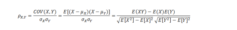
  当两个变量的线性关系增强时，相关系数趋于1或-1。正相关时趋于1，负相关时趋于-1。当两个变量独立时相关系统为0，但反之不成立。当Y和X服从联合正态分布时，其相互独立和不相关是等价的。
皮尔森相关系数的计算通过下面代码实现。

override def computeCorrelationMatrix(X: RDD[Vector]): Matrix = {
    val rowMatrix = new RowMatrix(X)
    //计算协方差矩阵
    val cov = rowMatrix.computeCovariance()
    computeCorrelationMatrixFromCovariance(cov)
  }
def computeCorrelationMatrixFromCovariance(covarianceMatrix: Matrix): Matrix = {
    val cov = covarianceMatrix.toBreeze.asInstanceOf[BDM[Double]]
    val n = cov.cols
    // 计算对角元素的标准差
    var i = 0
    while (i < n) {
      cov(i, i) = if (closeToZero(cov(i, i))) 0.0 else math.sqrt(cov(i, i))
      i +=1
    }
    // Loop through columns since cov is column major
    var j = 0
    var sigma = 0.0
    var containNaN = false
    while (j < n) {
      sigma = cov(j, j)
      i = 0
      while (i < j) {
        val corr = if (sigma == 0.0 || cov(i, i) == 0.0) {
          containNaN = true
          Double.NaN
        } else {
          //根据上文的公式计算，即cov(x,y)/(sigma_x * sigma_y)
          cov(i, j) / (sigma * cov(i, i))
        }
        cov(i, j) = corr
        cov(j, i) = corr
        i += 1
      }
      j += 1
    }
    // put 1.0 on the diagonals
    i = 0
    while (i < n) {
      cov(i, i) = 1.0
      i +=1
    }
    Matrices.fromBreeze(cov)
  }

2 斯皮尔曼相关系数

  使用皮尔森线性相关系数有2个局限：首先，必须假设数据是成对地从正态分布中取得的；其次，数据至少在逻辑范围内是等距的。对不服从正态分布的资料不符合使用矩相关系数来描述关联性。
此时可采用秩相关（rank correlation），也称等级相关，来描述两个变量之间的关联程度与方向。斯皮尔曼秩相关系数就是其中一种。

  斯皮尔曼秩相关系数定义为排序变量(ranked variables)之间的皮尔逊相关系数。对于大小为n的样本集，将原始的数据X_i和Y_i转换成排序变量rgX_i和rgY_i，然后按照皮尔森相关系数的计算公式进行计算。

  下面的代码将原始数据转换成了排序数据。

override def computeCorrelationMatrix(X: RDD[Vector]): Matrix = {
    // ((columnIndex, value), rowUid)
    //使用zipWithUniqueId产生的rowUid全局唯一
    val colBased = X.zipWithUniqueId().flatMap { case (vec, uid) =>
      vec.toArray.view.zipWithIndex.map { case (v, j) =>
        ((j, v), uid)
      }
    }
    // 通过(columnIndex, value)全局排序，排序的好处是使下面只需迭代一次
    val sorted = colBased.sortByKey()
    // 分配全局的ranks (using average ranks for tied values)
    val globalRanks = sorted.zipWithIndex().mapPartitions { iter =>
      var preCol = -1
      var preVal = Double.NaN
      var startRank = -1.0
      var cachedUids = ArrayBuffer.empty[Long]
      val flush: () => Iterable[(Long, (Int, Double))] = () => {
        val averageRank = startRank + (cachedUids.size - 1) / 2.0
        val output = cachedUids.map { uid =>
          (uid, (preCol, averageRank))
        }
        cachedUids.clear()
        output
      }
      iter.flatMap { case (((j, v), uid), rank) =>
        // 如果有新的值或者cachedUids过大, 调用flush
        if (j != preCol || v != preVal || cachedUids.size >= 10000000) {
          val output = flush()
          preCol = j
          preVal = v
          startRank = rank
          cachedUids += uid
          output
        } else {
          cachedUids += uid
          Iterator.empty
        }
      } ++ flush()
    } 
   //使用rank值代替原来的值
   val groupedRanks = globalRanks.groupByKey().map { case (uid, iter) =>
       // 根据列索引排序
       Vectors.dense(iter.toSeq.sortBy(_._1).map(_._2).toArray)
   }

  在每个分区内部，对于列索引相同且值相同的数据对，我们为其分配平均rank值。平均rank的计算方式如下面公式所示：

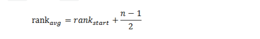
  其中rank_start表示列索引相同且值相同的数据对在分区中第一次出现时的索引位置，n表示列索引相同且值相同的数据对出现的次数。

3 参考文献

【1】Pearson product-moment correlation coefficient

【2】Spearman’s rank correlation coefficient

【3】相关性检验—Spearman秩相关系数和皮尔森相关系数

假设检测

  假设检测是统计中有力的工具，它用于判断一个结果是否在统计上是显著的、这个结果是否有机会发生。spark.mllib目前支持皮尔森卡方检测。输入属性的类型决定是作拟合优度(goodness of fit)检测还是作独立性检测。
拟合优度检测需要输入数据的类型是vector，独立性检测需要输入数据的类型是Matrix。

  spark.mllib也支持输入数据类型为RDD[LabeledPoint]，它用来通过卡方独立性检测作特征选择。Statistics提供方法用来作皮尔森卡方检测。下面是一个例子：

import org.apache.spark.SparkContext
import org.apache.spark.mllib.linalg._
import org.apache.spark.mllib.regression.LabeledPoint
import org.apache.spark.mllib.stat.Statistics._
val sc: SparkContext = ...
val vec: Vector = ... // a vector composed of the frequencies of events
// 作皮尔森拟合优度检测 
val goodnessOfFitTestResult = Statistics.chiSqTest(vec)
println(goodnessOfFitTestResult) 
val mat: Matrix = ... // a contingency matrix
// 作皮尔森独立性检测
val independenceTestResult = Statistics.chiSqTest(mat) 
println(independenceTestResult) // summary of the test including the p-value, degrees of freedom...
val obs: RDD[LabeledPoint] = ... // (feature, label) pairs.
// 独立性检测用于特征选择
val featureTestResults: Array[ChiSqTestResult] = Statistics.chiSqTest(obs)
var i = 1
featureTestResults.foreach { result =>
    println(s"Column $i:\n$result")
    i += 1
}

  另外，spark.mllib提供了一个Kolmogorov-Smirnov (KS)检测的1-sample, 2-sided实现，用来检测概率分布的相等性。通过提供理论分布（现在仅仅支持正太分布）的名字以及它相应的参数，
或者提供一个计算累积分布(cumulative distribution)的函数，用户可以检测原假设或零假设(null hypothesis)：即样本是否来自于这个分布。用户检测正太分布，但是不提供分布参数，检测会默认该分布为标准正太分布。

  Statistics提供了一个运行1-sample, 2-sided KS检测的方法，下面就是一个应用的例子。

import org.apache.spark.mllib.stat.Statistics
val data: RDD[Double] = ... // an RDD of sample data
// run a KS test for the sample versus a standard normal distribution
val testResult = Statistics.kolmogorovSmirnovTest(data, "norm", 0, 1)
println(testResult) 
// perform a KS test using a cumulative distribution function of our making
val myCDF: Double => Double = ...
val testResult2 = Statistics.kolmogorovSmirnovTest(data, myCDF)

流式显著性检测

  显著性检验即用于实验处理组与对照组或两种不同处理的效应之间是否有差异，以及这种差异是否显著的方法。

  常把一个要检验的假设记作H0,称为原假设（或零假设） (null hypothesis) ，与H0对立的假设记作H1，称为备择假设(alternative hypothesis) 。

• 在原假设为真时，决定放弃原假设，称为第一类错误，其出现的概率通常记作alpha
• 在原假设不真时，决定接受原假设，称为第二类错误，其出现的概率通常记作beta

  通常只限定犯第一类错误的最大概率alpha， 不考虑犯第二类错误的概率beta。这样的假设检验又称为显著性检验，概率alpha称为显著性水平。

  MLlib提供一些检测的在线实现，用于支持诸如A/B测试的场景。这些检测可能执行在Spark Streaming的DStream[(Boolean,Double)]上，元组的第一个元素表示控制组(control group (false))或者处理组(treatment group (true)),
第二个元素表示观察者的值。

  流式显著性检测支持下面的参数：

• peacePeriod：来自流中忽略的初始数据点的数量，用于减少novelty effects；
• windowSize：执行假设检测的以往批次的数量。如果设置为0，将对之前所有的批次数据作累积处理。

  StreamingTest支持流式假设检测。下面是一个应用的例子。

val data = ssc.textFileStream(dataDir).map(line => line.split(",") match {
  case Array(label, value) => BinarySample(label.toBoolean, value.toDouble)
})
val streamingTest = new StreamingTest()
  .setPeacePeriod(0)
  .setWindowSize(0)
  .setTestMethod("welch")
val out = streamingTest.registerStream(data)
out.print()

参考文献

【1】显著性检验

核密度估计

1 理论分析

  核密度估计是在概率论中用来估计未知的密度函数，属于非参数检验方法之一。假设我们有n个数，要计算某个数X的概率密度有多大，
可以通过下面的核密度估计方法估计。

  在上面的式子中，K为核密度函数，h为窗宽。核密度函数的原理比较简单，在我们知道某一事物的概率分布的情况下，如果某一个数在观察中出现了，我们可以认为这个数的概率密度很大，和这个数比较近的数的概率密度也会比较大，而那些离这个数远的数的概率密度会比较小。

  基于这种想法，针对观察中的第一个数，我们可以用K去拟合我们想象中的那个远小近大概率密度。对每一个观察数拟合出的多个概率密度分布函数，取平均。如果某些数是比较重要的，则可以取加权平均。需要说明的一点是，核密度的估计并不是找到真正的分布函数。

  在MLlib中，仅仅支持以高斯核做核密度估计。以高斯核做核密度估计时核密度估计公式（1）如下：

2 例子

  KernelDensity提供了方法通过样本RDD计算核密度估计。下面的例子给出了使用方法。

import org.apache.spark.mllib.stat.KernelDensity
import org.apache.spark.rdd.RDD
val data: RDD[Double] = ... // an RDD of sample data
// Construct the density estimator with the sample data and a standard deviation for the Gaussian
// kernels
val kd = new KernelDensity()
  .setSample(data)
  .setBandwidth(3.0)
// Find density estimates for the given values
val densities = kd.estimate(Array(-1.0, 2.0, 5.0))

3 代码实现

  通过调用KernelDensity.estimate方法来实现核密度函数估计。看下面的代码。

def estimate(points: Array[Double]): Array[Double] = {
    val sample = this.sample
    val bandwidth = this.bandwidth
    val n = points.length
    // 在每个高斯密度函数计算中，这个值都需要计算，所以提前计算。
    val logStandardDeviationPlusHalfLog2Pi = math.log(bandwidth) + 0.5 * math.log(2 * math.Pi)
    val (densities, count) = sample.aggregate((new Array[Double](n), 0L))(
      (x, y) => {
        var i = 0
        while (i < n) {
          x._1(i) += normPdf(y, bandwidth, logStandardDeviationPlusHalfLog2Pi, points(i))
          i += 1
        }
        (x._1, x._2 + 1)
      },
      (x, y) => {
        //daxpy函数的作用是将一个向量加上另一个向量的值，即：dy[i]+=da*dx[i]，其中da为常数
        blas.daxpy(n, 1.0, y._1, 1, x._1, 1)
        (x._1, x._2 + y._2)
      })
    //在向量上乘一个常数
    blas.dscal(n, 1.0 / count, densities, 1)
    densities
  }
}

  上述代码的seqOp函数中调用了normPdf，这个函数用于计算核函数为高斯分布的概率密度函数。参见上面的公式(1)。公式(1)的实现如下面代码。

 def normPdf(
      mean: Double,
      standardDeviation: Double,
      logStandardDeviationPlusHalfLog2Pi: Double,
      x: Double): Double = {
    val x0 = x - mean
    val x1 = x0 / standardDeviation
    val logDensity = -0.5 * x1 * x1 - logStandardDeviationPlusHalfLog2Pi
    math.exp(logDensity)
  }

  该方法首先将公式(1)取对数，计算结果，然后再对计算结果取指数。

参考文献

【1】核密度估计

【2】R语言与非参数统计（核密度估计）

随机数生成

  随机数生成在随机算法、性能测试中非常有用，spark.mllib支持生成随机的RDD,RDD的独立同分布(iid)的值来自于给定的分布：均匀分布、标准正太分布、泊松分布。

  RandomRDDs提供工厂方法生成随机的双精度RDD或者向量RDD。下面的例子生成了一个随机的双精度RDD，它的值来自于标准的正太分布N(0,1)。

import org.apache.spark.SparkContext
import org.apache.spark.mllib.random.RandomRDDs._
val sc: SparkContext = ...
// Generate a random double RDD that contains 1 million i.i.d. values drawn from the
// standard normal distribution `N(0, 1)`, evenly distributed in 10 partitions.
val u = normalRDD(sc, 1000000L, 10)
// Apply a transform to get a random double RDD following `N(1, 4)`.
val v = u.map(x => 1.0 + 2.0 * x)

  normalRDD的实现如下面代码所示。

def normalRDD(
      sc: SparkContext,
      size: Long,
      numPartitions: Int = 0,
      seed: Long = Utils.random.nextLong()): RDD[Double] = {
    val normal = new StandardNormalGenerator()
    randomRDD(sc, normaal, size, numPartitionsOrDefault(sc, numPartitions), seed)
  }
def randomRDD[T: ClassTag](
      sc: SparkContext,
      generator: RandomDataGenerator[T],
      size: Long,
      numPartitions: Int = 0,
      seed: Long = Utils.random.nextLong()): RDD[T] = {
    new RandomRDD[T](sc, size, numPartitionsOrDefault(sc, numPartitions), generator, seed)
  }
private[mllib] class RandomRDD[T: ClassTag](sc: SparkContext,
    size: Long,
    numPartitions: Int,
    @transient private val rng: RandomDataGenerator[T],
    @transient private val seed: Long = Utils.random.nextLong) extends RDD[T](sc, Nil)

概括统计

  MLlib支持RDD[Vector]列的概括统计，它通过调用Statistics的colStats方法实现。colStats返回一个MultivariateStatisticalSummary对象，这个对象包含列式的最大值、最小值、均值、方差等等。
下面是一个应用例子：

import org.apache.spark.mllib.linalg.Vector
import org.apache.spark.mllib.stat.{MultivariateStatisticalSummary, Statistics}
val observations: RDD[Vector] = ... // an RDD of Vectors
// Compute column summary statistics.
val summary: MultivariateStatisticalSummary = Statistics.colStats(observations)
println(summary.mean) // a dense vector containing the mean value for each column
println(summary.variance) // column-wise variance
println(summary.numNonzeros) // number of nonzeros in each column

  下面我们具体看看colStats方法的实现。

def colStats(X: RDD[Vector]): MultivariateStatisticalSummary = {
    new RowMatrix(X).computeColumnSummaryStatistics()
  }

  上面的代码非常明显，利用传人的RDD创建RowMatrix对象，利用方法computeColumnSummaryStatistics统计指标。

def computeColumnSummaryStatistics(): MultivariateStatisticalSummary = {
    val summary = rows.treeAggregate(new MultivariateOnlineSummarizer)(
      (aggregator, data) => aggregator.add(data),
      (aggregator1, aggregator2) => aggregator1.merge(aggregator2))
    updateNumRows(summary.count)
    summary
  }

  上面的代码调用了RDD的treeAggregate方法，treeAggregate是聚合方法，它迭代处理RDD中的数据，其中，(aggregator, data) => aggregator.add(data)处理每条数据，将其添加到MultivariateOnlineSummarizer，
(aggregator1, aggregator2) => aggregator1.merge(aggregator2)将不同分区的MultivariateOnlineSummarizer对象汇总。所以上述代码实现的重点是add方法和merge方法。它们都定义在MultivariateOnlineSummarizer中。
我们先来看add代码。

@Since("1.1.0")
  def add(sample: Vector): this.type = add(sample, 1.0)
  private[spark] def add(instance: Vector, weight: Double): this.type = {
    if (weight == 0.0) return this
    if (n == 0) {
      n = instance.size
      currMean = Array.ofDim[Double](n)
      currM2n = Array.ofDim[Double](n)
      currM2 = Array.ofDim[Double](n)
      currL1 = Array.ofDim[Double](n)
      nnz = Array.ofDim[Double](n)
      currMax = Array.fill[Double](n)(Double.MinValue)
      currMin = Array.fill[Double](n)(Double.MaxValue)
    }
    val localCurrMean = currMean
    val localCurrM2n = currM2n
    val localCurrM2 = currM2
    val localCurrL1 = currL1
    val localNnz = nnz
    val localCurrMax = currMax
    val localCurrMin = currMin
    instance.foreachActive { (index, value) =>
      if (value != 0.0) {
        if (localCurrMax(index) < value) {
          localCurrMax(index) = value
        }
        if (localCurrMin(index) > value) {
          localCurrMin(index) = value
        }
        val prevMean = localCurrMean(index)
        val diff = value - prevMean
        localCurrMean(index) = prevMean + weight * diff / (localNnz(index) + weight)
        localCurrM2n(index) += weight * (value - localCurrMean(index)) * diff
        localCurrM2(index) += weight * value * value
        localCurrL1(index) += weight * math.abs(value)
        localNnz(index) += weight
      }
    }
    weightSum += weight
    weightSquareSum += weight * weight
    totalCnt += 1
    this
  }

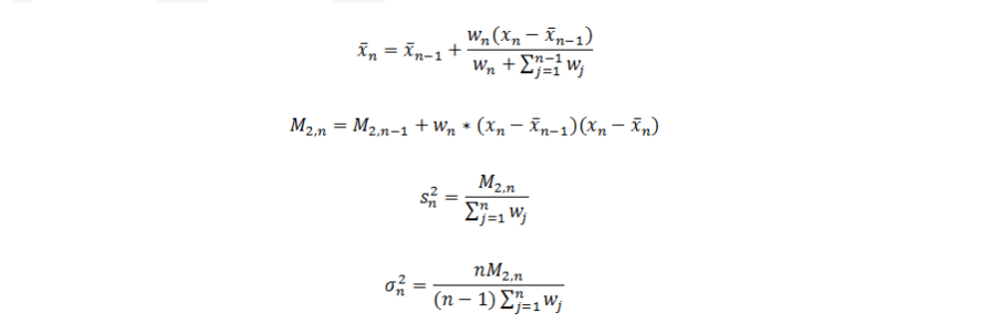
  这段代码使用了在线算法来计算均值和方差。根据文献【1】的介绍，计算均值和方差遵循如下的迭代公式：

  在上面的公式中，x表示样本均值，s表示样本方差，delta表示总体方差。MLlib实现的是带有权重的计算，所以使用的迭代公式略有不同，参考文献【2】。

  merge方法相对比较简单，它只是对两个MultivariateOnlineSummarizer对象的指标作合并操作。

 def merge(other: MultivariateOnlineSummarizer): this.type = {
    if (this.weightSum != 0.0 && other.weightSum != 0.0) {
      totalCnt += other.totalCnt
      weightSum += other.weightSum
      weightSquareSum += other.weightSquareSum
      var i = 0
      while (i < n) {
        val thisNnz = nnz(i)
        val otherNnz = other.nnz(i)
        val totalNnz = thisNnz + otherNnz
        if (totalNnz != 0.0) {
          val deltaMean = other.currMean(i) - currMean(i)
          // merge mean together
          currMean(i) += deltaMean * otherNnz / totalNnz
          // merge m2n together，不单纯是累加
          currM2n(i) += other.currM2n(i) + deltaMean * deltaMean * thisNnz * otherNnz / totalNnz
          // merge m2 together
          currM2(i) += other.currM2(i)
          // merge l1 together
          currL1(i) += other.currL1(i)
          // merge max and min
          currMax(i) = math.max(currMax(i), other.currMax(i))
          currMin(i) = math.min(currMin(i), other.currMin(i))
        }
        nnz(i) = totalNnz
        i += 1
      }
    } else if (weightSum == 0.0 && other.weightSum != 0.0) {
      this.n = other.n
      this.currMean = other.currMean.clone()
      this.currM2n = other.currM2n.clone()
      this.currM2 = other.currM2.clone()
      this.currL1 = other.currL1.clone()
      this.totalCnt = other.totalCnt
      this.weightSum = other.weightSum
      this.weightSquareSum = other.weightSquareSum
      this.nnz = other.nnz.clone()
      this.currMax = other.currMax.clone()
      this.currMin = other.currMin.clone()
    }
    this
  }

  这里需要注意的是，在线算法的并行化实现是一种特殊情况。例如样本集X分到两个不同的分区，分别为X_A和X_B，那么它们的合并需要满足下面的公式：

  依靠文献【3】我们可以知道，样本方差的无偏估计由下面的公式给出：

  所以，真实的样本均值和样本方差通过下面的代码实现。

override def mean: Vector = {
    val realMean = Array.ofDim[Double](n)
    var i = 0
    while (i < n) {
      realMean(i) = currMean(i) * (nnz(i) / weightSum)
      i += 1
    }
    Vectors.dense(realMean)
  }
 override def variance: Vector = {
    val realVariance = Array.ofDim[Double](n)
    val denominator = weightSum - (weightSquareSum / weightSum)
    // Sample variance is computed, if the denominator is less than 0, the variance is just 0.
    if (denominator > 0.0) {
      val deltaMean = currMean
      var i = 0
      val len = currM2n.length
      while (i < len) {
        realVariance(i) = (currM2n(i) + deltaMean(i) * deltaMean(i) * nnz(i) *
          (weightSum - nnz(i)) / weightSum) / denominator
        i += 1
      }
    }
    Vectors.dense(realVariance)
  }

参考文献

【1】Algorithms for calculating variance

【2】Updating mean and variance estimates: an improved method

【3】Weighted arithmetic mean

分层取样

  先将总体的单位按某种特征分为若干次级总体（层），然后再从每一层内进行单纯随机抽样，组成一个样本的统计学计算方法叫做分层抽样。在spark.mllib中，用key来分层。

  与存在于spark.mllib中的其它统计函数不同，分层采样方法sampleByKey和sampleByKeyExact可以在key-value对的RDD上执行。在分层采样中，可以认为key是一个标签，
value是特定的属性。例如，key可以是男人或者女人或者文档id,它相应的value可能是一组年龄或者是文档中的词。sampleByKey方法通过掷硬币的方式决定是否采样一个观察数据，
因此它需要我们传递（pass over）数据并且提供期望的数据大小(size)。sampleByKeyExact比每层使用sampleByKey随机抽样需要更多的有意义的资源，但是它能使样本大小的准确性达到了99.99%。

  sampleByKeyExact()允许用户准确抽取f_k * n_k个样本，
这里f_k表示期望获取键为k的样本的比例，n_k表示键为k的键值对的数量。下面是一个使用的例子：

import org.apache.spark.SparkContext
import org.apache.spark.SparkContext._
import org.apache.spark.rdd.PairRDDFunctions
val sc: SparkContext = ...
val data = ... // an RDD[(K, V)] of any key value pairs
val fractions: Map[K, Double] = ... // specify the exact fraction desired from each key
// Get an exact sample from each stratum
val approxSample = data.sampleByKey(withReplacement = false, fractions)
val exactSample = data.sampleByKeyExact(withReplacement = false, fractions)

  当withReplacement为true时，采用PoissonSampler取样器，当withReplacement为false使，采用BernoulliSampler取样器。

def sampleByKey(withReplacement: Boolean,
      fractions: Map[K, Double],
      seed: Long = Utils.random.nextLong): RDD[(K, V)] = self.withScope {
    val samplingFunc = if (withReplacement) {
      StratifiedSamplingUtils.getPoissonSamplingFunction(self, fractions, false, seed)
    } else {
      StratifiedSamplingUtils.getBernoulliSamplingFunction(self, fractions, false, seed)
    }
    self.mapPartitionsWithIndex(samplingFunc, preservesPartitioning = true)
  }
def sampleByKeyExact(
      withReplacement: Boolean,
      fractions: Map[K, Double],
      seed: Long = Utils.random.nextLong): RDD[(K, V)] = self.withScope {
    val samplingFunc = if (withReplacement) {
      StratifiedSamplingUtils.getPoissonSamplingFunction(self, fractions, true, seed)
    } else {
      StratifiedSamplingUtils.getBernoulliSamplingFunction(self, fractions, true, seed)
    }
    self.mapPartitionsWithIndex(samplingFunc, preservesPartitioning = true)
  }

  下面我们分别来看sampleByKey和sampleByKeyExact的实现。

1 sampleByKey的实现

  当我们需要不重复抽样时，我们需要用泊松抽样器来抽样。当需要重复抽样时，用伯努利抽样器抽样。sampleByKey的实现比较简单，它就是统一的随机抽样。

1.1 泊松抽样器

  我们首先看泊松抽样器的实现。

def getPoissonSamplingFunction[K: ClassTag, V: ClassTag](rdd: RDD[(K, V)],
      fractions: Map[K, Double],
      exact: Boolean,
      seed: Long): (Int, Iterator[(K, V)]) => Iterator[(K, V)] = {
      (idx: Int, iter: Iterator[(K, V)]) => {
              //初始化随机生成器
              val rng = new RandomDataGenerator()
              rng.reSeed(seed + idx)
              iter.flatMap { item =>
                //获得下一个泊松值
                val count = rng.nextPoisson(fractions(item._1))
                if (count == 0) {
                  Iterator.empty
                } else {
                  Iterator.fill(count)(item)
                }
              }
            }
}

  getPoissonSamplingFunction返回的是一个函数，传递给mapPartitionsWithIndex处理每个分区的数据。这里RandomDataGenerator是一个随机生成器，它用于同时生成均匀值(uniform values)和泊松值(Poisson values)。

1.2 伯努利抽样器

def getBernoulliSamplingFunction[K, V](rdd: RDD[(K, V)],
      fractions: Map[K, Double],
      exact: Boolean,
      seed: Long): (Int, Iterator[(K, V)]) => Iterator[(K, V)] = {
    var samplingRateByKey = fractions
    (idx: Int, iter: Iterator[(K, V)]) => {
      //初始化随机生成器
      val rng = new RandomDataGenerator()
      rng.reSeed(seed + idx)
      // Must use the same invoke pattern on the rng as in getSeqOp for without replacement
      // in order to generate the same sequence of random numbers when creating the sample
      iter.filter(t => rng.nextUniform() < samplingRateByKey(t._1))
    }
  }

2 sampleByKeyExact的实现

  sampleByKeyExact获取更准确的抽样结果，它的实现也分为两种情况，重复抽样和不重复抽样。前者使用泊松抽样器，后者使用伯努利抽样器。

2.1 泊松抽样器

val counts = Some(rdd.countByKey())
//计算立即接受的样本数量，并且为每层生成候选名单
val finalResult = getAcceptanceResults(rdd, true, fractions, counts, seed)
//决定接受样本的阈值，生成准确的样本大小
val thresholdByKey = computeThresholdByKey(finalResult, fractions)
(idx: Int, iter: Iterator[(K, V)]) => {
     val rng = new RandomDataGenerator()
     rng.reSeed(seed + idx)
     iter.flatMap { item =>
          val key = item._1
          val acceptBound = finalResult(key).acceptBound
          // Must use the same invoke pattern on the rng as in getSeqOp for with replacement
          // in order to generate the same sequence of random numbers when creating the sample
          val copiesAccepted = if (acceptBound == 0) 0L else rng.nextPoisson(acceptBound)
          //候选名单
          val copiesWaitlisted = rng.nextPoisson(finalResult(key).waitListBound)
          val copiesInSample = copiesAccepted +
            (0 until copiesWaitlisted).count(i => rng.nextUniform() < thresholdByKey(key))
          if (copiesInSample > 0) {
            Iterator.fill(copiesInSample.toInt)(item)
          } else {
            Iterator.empty
          }
     }
}

2.2 伯努利抽样

def getBernoulliSamplingFunction[K, V](rdd: RDD[(K, V)],
      fractions: Map[K, Double],
      exact: Boolean,
      seed: Long): (Int, Iterator[(K, V)]) => Iterator[(K, V)] = {
    var samplingRateByKey = fractions
    //计算立即接受的样本数量，并且为每层生成候选名单
    val finalResult = getAcceptanceResults(rdd, false, fractions, None, seed)
    //决定接受样本的阈值，生成准确的样本大小
    samplingRateByKey = computeThresholdByKey(finalResult, fractions)
    (idx: Int, iter: Iterator[(K, V)]) => {
      val rng = new RandomDataGenerator()
      rng.reSeed(seed + idx)
      // Must use the same invoke pattern on the rng as in getSeqOp for without replacement
      // in order to generate the same sequence of random numbers when creating the sample
      iter.filter(t => rng.nextUniform() < samplingRateByKey(t._1))
    }
  }