第四章 训练模型

# Python ≥3.5 is required
import sys
assert sys.version_info >= (3, 5)
# Scikit-Learn ≥0.20 is required
import sklearn
assert sklearn.__version__ >= "0.20"
# Common imports
import numpy as np
import os
# to make this notebook's output stable across runs
np.random.seed(42)
# To plot pretty figures
%matplotlib inline
import matplotlib as mpl
import matplotlib.pyplot as plt
mpl.rc('axes', labelsize=14)
mpl.rc('xtick', labelsize=12)
mpl.rc('ytick', labelsize=12)
# Where to save the figures
PROJECT_ROOT_DIR = "."
CHAPTER_ID = "training_linear_models"
IMAGES_PATH = os.path.join(PROJECT_ROOT_DIR, "images", CHAPTER_ID)
# os.makedirs(IMAGES_PATH, exist_ok=True)
def save_fig(fig_id, tight_layout=True, fig_extension="png", resolution=300):
    path = os.path.join(IMAGES_PATH, fig_id + "." + fig_extension)
    print("Saving figure", fig_id)
    if tight_layout:
        plt.tight_layout()
    plt.savefig(path, format=fig_extension, dpi=resolution)
# Ignore useless warnings (see SciPy issue #5998)
import warnings
warnings.filterwarnings(action="ignore", message="^internal gelsd")

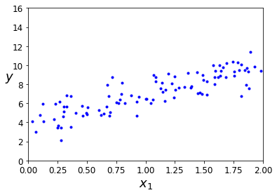
import numpy as np
X = 2 * np.random.rand(100, 1)
y = 4 + 3 * X + np.random.randn(100, 1)

plt.plot(X, y, "b.")
plt.xlabel("$x_1$", fontsize=18)
plt.ylabel("$y$", rotation=0, fontsize=18)
plt.axis([0, 2, 0, 16])
# save_fig("generated_data_plot")
plt.show()

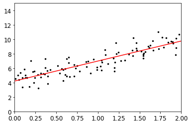
1.使用标准方程计算出theta

X_b = np.c_[np.ones((100,1)),X]
X_b
theta_best = np.linalg.inv(X_b.T.dot(X_b)).dot(X_b.T).dot(y)
theta_best

X_new = np.array([[0],[2]])
X_new_b = np.c_[np.ones((2,1)),X_new]
y_predict = X_new_b.dot(theta_best)
y_predict

plt.plot(X_new,y_predict,'r-')
plt.scatter(X,y,c='k',s=6)
plt.axis([0,2,0,15])
plt.show()

2.使用sklearn

from sklearn.linear_model import LinearRegression
lin_reg = LinearRegression()
lin_reg.fit(X,y)
lin_reg.intercept_ , lin_reg.coef_
lin_reg.predict(X_new)

3.梯度下降法的快速实现

eta = 0.1  # learning rate
n_iterations = 1000
m = 100
theta = np.random.randn(2,1)  # random initialization
for iteration in range(n_iterations):
    gradients = 2/m * X_b.T.dot(X_b.dot(theta) - y)
    theta = theta - eta * gradients

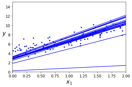
4.随机梯度下降的快速实现

theta_path_sgd = []
m = len(X_b)
np.random.seed(42)
n_epochs = 50
t0, t1 = 5, 50  # learning schedule hyperparameters
def learning_schedule(t):
    return t0 / (t + t1)
theta = np.random.randn(2,1)  # random initialization
for epoch in range(n_epochs):
    for i in range(m):
        if epoch == 0 and i < 20:                    
            y_predict = X_new_b.dot(theta)           
            style = "b-" if i > 0 else "r--"         
            plt.plot(X_new, y_predict, style)     
        random_index = np.random.randint(m)
        xi = X_b[random_index:random_index+1]
        yi = y[random_index:random_index+1]
        gradients = 2 * xi.T.dot(xi.dot(theta) - yi)
        eta = learning_schedule(epoch * m + i)
        theta = theta - eta * gradients
        theta_path_sgd.append(theta)                 
plt.plot(X, y, "b.")                                 
plt.xlabel("$x_1$", fontsize=18)                    
plt.ylabel("$y$", rotation=0, fontsize=18)          
plt.axis([0, 2, 0, 15])                            
save_fig("sgd_plot")                              
plt.show()

5.多项式回归

利用sklearn.preprocessing的PolynomialFeatures添加新特征，再用LinearRegression拟合。

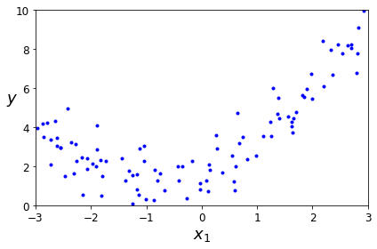
import numpy as np
import numpy.random as rnd
np.random.seed(42)
m = 100
X = 6 * np.random.rand(m, 1) - 3
y = 0.5 * X**2 + X + 2 + np.random.randn(m, 1)
plt.plot(X, y, "b.")
plt.xlabel("$x_1$", fontsize=18)
plt.ylabel("$y$", rotation=0, fontsize=18)
plt.axis([-3, 3, 0, 10])
plt.show()

from sklearn.preprocessing import PolynomialFeatures
poly_features = PolynomialFeatures(degree=2, include_bias=False)
X_poly = poly_features.fit_transform(X)
X[0]

lin_reg = LinearRegression()
lin_reg.fit(X_poly, y)
lin_reg.intercept_, lin_reg.coef_

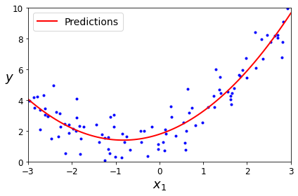
X_new=np.linspace(-3, 3, 100).reshape(100, 1)
X_new_poly = poly_features.transform(X_new)
y_new = lin_reg.predict(X_new_poly)
plt.plot(X, y, "b.")
plt.plot(X_new, y_new, "r-", linewidth=2, label="Predictions")
plt.xlabel("$x_1$", fontsize=18)
plt.ylabel("$y$", rotation=0, fontsize=18)
plt.legend(loc="upper left", fontsize=14)
plt.axis([-3, 3, 0, 10])
plt.show()

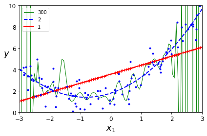
变换degree为1，2，300.

from sklearn.preprocessing import StandardScaler
from sklearn.pipeline import Pipeline
for style, width, degree in (("g-", 1, 300), ("b--", 2, 2), ("r-+", 2, 1)):
    polybig_features = PolynomialFeatures(degree=degree, include_bias=False)
    std_scaler = StandardScaler()
    lin_reg = LinearRegression()
    polynomial_regression = Pipeline([
            ("poly_features", polybig_features),
            ("std_scaler", std_scaler),
            ("lin_reg", lin_reg),
        ])
    polynomial_regression.fit(X, y)
    y_newbig = polynomial_regression.predict(X_new)
    plt.plot(X_new, y_newbig, style, label=str(degree), linewidth=width)
plt.plot(X, y, "b.", linewidth=3)
plt.legend(loc="upper left")
plt.xlabel("$x_1$", fontsize=18)
plt.ylabel("$y$", rotation=0, fontsize=18)
plt.axis([-3, 3, 0, 10])
plt.show()

6.学习曲线

欠拟合曲线与过拟合曲线
偏差/方差权衡

7.正则化

7.1 岭回归

from sklearn.linear_model import Ridge
ridge_reg = Ridge(alpha=1, solver="cholesky", random_state=42)
ridge_reg.fit(X, y)
ridge_reg.predict([[1.5]])

7.2Lasso回归

Lasso回归的一个重要特点是它倾向于完全消除掉最不重要特征的权重(也就是将它设置为0)

7.3弹性网络

弹性网络是介于岭回归和Lasso回归之间的中间地带。正则项是Ridge和Lasso正则项的简单混合。
一般而言，弹性网络优于Lasso回归，因为当特征数量超过训练实例数量，又或者是几个特征强相关时，Lasso回归的表现可能非常不稳定。sklearn中为ElasticNet

7.4提前停止

对于梯度下降这一类迭代算法，还有一个与众不同的正则化方法，就是在验证误差达到最小值时停止训练，该方法叫做提前停止法。

8.逻辑回归

8.1 Softmax回归

Softmax回归分类器一次只能预测一个类，因此它只能与互斥的类一起使用。无法使用它在一张照片中识别多个人。