激活函数的使用
首先导入我们需要的包:
其中torch.nn.functional中的nn是神经网络模块
通过pytorch计算各个激活函数的值: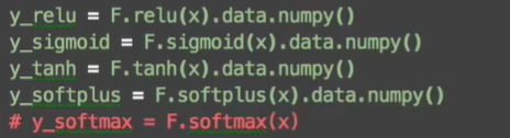
最后使用matpplotlib画出来:
Regression(回归)
import torchimport torch.nn.functional as Fimport matplotlib.pyplot as pltx = torch.unsqueeze(torch.linspace(-1, 1, 100), dim=1) # x data (tensor), shape=(100, 1) 自己定义的数据y = x.pow(2) + 0.2*torch.rand(x.size()) # noisy y data (tensor), shape=(100, 1) 自己定义的函数# torch can only train on Variable, so convert them to Variable# The code below is deprecated in Pytorch 0.4. Now, autograd directly supports tensors# x, y = Variable(x), Variable(y)# plt.scatter(x.data.numpy(), y.data.numpy())# plt.show()class Net(torch.nn.Module): #用class来定义neural networkdef __init__(self, n_feature, n_hidden, n_output): #其中包含了初始化层所需要的信息super(Net, self).__init__()self.hidden = torch.nn.Linear(n_feature, n_hidden) # hidden layerself.predict = torch.nn.Linear(n_hidden, n_output) # output layerdef forward(self, x): #network中前一项传递的过程x = F.relu(self.hidden(x)) # activation function for hidden layerx = self.predict(x) # linear outputreturn xnet = Net(n_feature=1, n_hidden=10, n_output=1) # define the networkprint(net) # net architectureoptimizer = torch.optim.SGD(net.parameters(), lr=0.2) #使用SGD方法对我们的函数进行优化,net.parameters()是net中所有的参数,lr是learning rate学习效率(不宜太低或太高)loss_func = torch.nn.MSELoss() # this is for regression mean squared loss 主要用于回归问题,与分类问题不同plt.ion() # something about plottingfor t in range(200):prediction = net(x) # input x and predict based on xloss = loss_func(prediction, y) # must be (1. nn output, 2. target)optimizer.zero_grad() # clear gradients for next trainloss.backward() # backpropagation, compute gradientsoptimizer.step() # apply gradients 更新参数if t % 5 == 0:# plot and show learning processplt.cla()plt.scatter(x.data.numpy(), y.data.numpy())plt.plot(x.data.numpy(), prediction.data.numpy(), 'r-', lw=5)plt.text(0.5, 0, 'Loss=%.4f' % loss.data.numpy(), fontdict={'size': 20, 'color': 'red'})plt.pause(0.1)plt.ioff()plt.show()
Classification(分类)
import torchimport torch.nn.functional as Fimport matplotlib.pyplot as plt# torch.manual_seed(1) # reproducible# 自己制作的假的数据n_data = torch.ones(100, 2)x0 = torch.normal(2*n_data, 1) # class0 x data (tensor), shape=(100, 2)y0 = torch.zeros(100) # class0 y data (tensor), shape=(100, 1)x1 = torch.normal(-2*n_data, 1) # class1 x data (tensor), shape=(100, 2)y1 = torch.ones(100) # class1 y data (tensor), shape=(100, 1)x = torch.cat((x0, x1), 0).type(torch.FloatTensor) # shape (200, 2) FloatTensor = 32-bit floatingy = torch.cat((y0, y1), ).type(torch.LongTensor) # shape (200,) LongTensor = 64-bit integer# The code below is deprecated in Pytorch 0.4. Now, autograd directly supports tensors# x, y = Variable(x), Variable(y)# plt.scatter(x.data.numpy()[:, 0], x.data.numpy()[:, 1], c=y.data.numpy(), s=100, lw=0, cmap='RdYlGn')# plt.show()class Net(torch.nn.Module):def __init__(self, n_feature, n_hidden, n_output):super(Net, self).__init__()self.hidden = torch.nn.Linear(n_feature, n_hidden) # hidden layerself.out = torch.nn.Linear(n_hidden, n_output) # output layerdef forward(self, x):x = F.relu(self.hidden(x)) # activation function for hidden layerx = self.out(x)return xnet = Net(n_feature=2, n_hidden=10, n_output=2) # define the networkprint(net) # net architectureoptimizer = torch.optim.SGD(net.parameters(), lr=0.02)loss_func = torch.nn.CrossEntropyLoss() # 主要用于分类问题计算lossplt.ion() # something about plottingfor t in range(100):out = net(x) # input x and predict based on xloss = loss_func(out, y) # must be (1. nn output, 2. target), the target label is NOT one-hottedoptimizer.zero_grad() # clear gradients for next trainloss.backward() # backpropagation, compute gradientsoptimizer.step() # apply gradientsif t % 2 == 0:# plot and show learning processplt.cla()prediction = torch.max(out, 1)[1]pred_y = prediction.data.numpy()target_y = y.data.numpy()plt.scatter(x.data.numpy()[:, 0], x.data.numpy()[:, 1], c=pred_y, s=100, lw=0, cmap='RdYlGn')accuracy = float((pred_y == target_y).astype(int).sum()) / float(target_y.size)plt.text(1.5, -4, 'Accuracy=%.2f' % accuracy, fontdict={'size': 20, 'color': 'red'})plt.pause(0.1)plt.ioff()plt.show()
快速搭建神经网络
class Net(torch.nn.Module):def __init__(self, n_feature, n_hidden, n_output):super(Net, self).__init__()self.hidden = torch.nn.Linear(n_feature, n_hidden) # hidden layerself.predict = torch.nn.Linear(n_hidden, n_output) # output layerdef forward(self, x):x = F.relu(self.hidden(x)) # activation function for hidden layerx = self.predict(x) # linear outputreturn xnet1 = Net(1, 10, 1)net2 = torch.nn.Sequential(torch.nn.Linear(1, 10),torch.nn.ReLU(),torch.nn.Linear(10, 1))

保存和提取神经网络
import torchimport matplotlib.pyplot as plt# torch.manual_seed(1) # reproducible# fake datax = torch.unsqueeze(torch.linspace(-1, 1, 100), dim=1) # x data (tensor), shape=(100, 1)y = x.pow(2) + 0.2*torch.rand(x.size()) # noisy y data (tensor), shape=(100, 1)# The code below is deprecated in Pytorch 0.4. Now, autograd directly supports tensors# x, y = Variable(x, requires_grad=False), Variable(y, requires_grad=False)def save():# save net1net1 = torch.nn.Sequential(torch.nn.Linear(1, 10),torch.nn.ReLU(),torch.nn.Linear(10, 1))optimizer = torch.optim.SGD(net1.parameters(), lr=0.5)loss_func = torch.nn.MSELoss()#训练for t in range(100):prediction = net1(x)loss = loss_func(prediction, y)optimizer.zero_grad()loss.backward()optimizer.step()# plot resultplt.figure(1, figsize=(10, 3))plt.subplot(131)plt.title('Net1')plt.scatter(x.data.numpy(), y.data.numpy())plt.plot(x.data.numpy(), prediction.data.numpy(), 'r-', lw=5)# 2 ways to save the nettorch.save(net1, 'net.pkl') # 保存整个神经网络torch.save(net1.state_dict(), 'net_params.pkl') # 保存神经网络中的参数def restore_net():# 提取net1并赋给net2net2 = torch.load('net.pkl')prediction = net2(x)# plot resultplt.subplot(132)plt.title('Net2')plt.scatter(x.data.numpy(), y.data.numpy())plt.plot(x.data.numpy(), prediction.data.numpy(), 'r-', lw=5)def restore_params():# 提取net1中的参数赋值给net3,首先要创建一个和net1相同结构的net3,再进行赋值net3 = torch.nn.Sequential(torch.nn.Linear(1, 10),torch.nn.ReLU(),torch.nn.Linear(10, 1))# 对net3进行赋值net3.load_state_dict(torch.load('net_params.pkl'))prediction = net3(x)# plot resultplt.subplot(133)plt.title('Net3')plt.scatter(x.data.numpy(), y.data.numpy())plt.plot(x.data.numpy(), prediction.data.numpy(), 'r-', lw=5)plt.show()# save net1save()# restore entire net (may slow)restore_net()# restore only the net parametersrestore_params()
批处理
import torchimport torch.utils.data as Datatorch.manual_seed(1) # reproducibleBATCH_SIZE = 5# BATCH_SIZE = 8x = torch.linspace(1, 10, 10) # this is x data (torch tensor)y = torch.linspace(10, 1, 10) # this is y data (torch tensor)torch_dataset = Data.TensorDataset(x, y)loader = Data.DataLoader(dataset=torch_dataset, # torch TensorDataset formatbatch_size=BATCH_SIZE, # 在一个epoch中每次batch读取多少个数据shuffle=True, # 是否要打乱进行读取num_workers=2, # subprocesses for loading data)def show_batch():for epoch in range(3): #全部数据共训练3次for step, (batch_x, batch_y) in enumerate(loader): # for each training step# train your data...print('Epoch: ', epoch, '| Step: ', step, '| batch x: ',batch_x.numpy(), '| batch y: ', batch_y.numpy())if __name__ == '__main__':show_batch()
当BATCH_SIZE=5,shuffle = Ture时: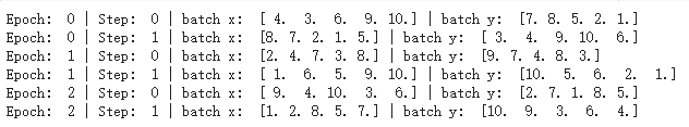
当BATCH_SIZE=8,shuffle = Fause时:

若有收获,就点个赞吧
0 人点赞
