这里的无脑只是分了组之后,对目的基因没有要求的情况下
因为DESeq2也涉及阈值设定,不一定确保目的基因一定在UP或者DN的基因里
这里也只是打包了DEG和GO_KEGG
加载R包及数据载入
library(DESeq2)library(ggplot2)library(ggrepel)library(pheatmap)library(clusterProfiler)library(org.Hs.eg.db)library(stringr)library(RColorBrewer)library(glmnet)library(ROCR)library(caret)library(timeROC)library(GSEABase)library(forcats)library(ggstance)library(RColorBrewer)load('Rdata/train_exp_cl.Rdata')group = factor(cl$risk1, levels = c('LowRisk', 'HighRisk'))
(一)差异分析
整理好表达矩阵exp和分组group,打包跑就行
DEG_DESeq2 = function(exp, group){colData <- data.frame(row.names =colnames(exp),condition=group)dds <- DESeqDataSetFromMatrix(countData = exp,colData = colData,design = ~ condition)dds <- DESeq(dds)res <- results(dds, contrast = c("condition",rev(levels(group))))resOrdered <- res[order(res$pvalue),]DEG <- as.data.frame(resOrdered)DEG = na.omit(DEG)logFC_cutoff <- with(DEG,mean(abs(log2FoldChange)) + 2*sd(abs(log2FoldChange)) )k1 = (DEG$pvalue < 0.05)&(DEG$log2FoldChange < -logFC_cutoff)k2 = (DEG$pvalue < 0.05)&(DEG$log2FoldChange > logFC_cutoff)DEG$change = ifelse(k1,"DOWN",ifelse(k2,"UP","NOT"))write.csv(DEG, file = 'outport/DEG_DESeq2.csv')}DEG_DESeq2(exp, group)DEG = read.csv('outport/DEG_DESeq2.csv')table(DEG$change)
(二)火山图
注释数据需要自己搞
# 一些火山图上的注释数据logFC_cutoff <- with(DEG,mean(abs(log2FoldChange)) + 2*sd(abs(log2FoldChange)) )DEG$label = ifelse(DEG$X == 'HMOX1', 'HMOX1', '')p1 = ggplot(DEG, aes(x=log2FoldChange, y=-log10(pvalue),color=change))+geom_point(alpha=0.5, size=1.8)+theme_set(theme_set(theme_bw(base_size=20)))+xlab("log2FC") + ylab("-log10(pvalue)")+scale_colour_manual(values = c("#377EB8",'grey', "#E41A1C"))+theme_classic()+theme(panel.border = element_rect(fill=NA,color="black", size=1, linetype="solid"))+geom_hline(aes(yintercept = -log10(0.05)), linetype = 'dashed', size = 1)+geom_vline(aes(xintercept = logFC_cutoff), linetype = 'dashed',size = 1)+geom_vline(aes(xintercept = -logFC_cutoff), linetype = 'dashed', size = 1)+geom_label_repel(aes(label = label))p1
(三)热图
注释数据需要自己搞
想看画图代码直接拖到最后p2
gene = c(DEG[DEG$change == 'UP','X'], DEG[DEG$change == 'DOWN','X'])data = log2(edgeR::cpm(exp)+1)[gene,]cl = cl[order(cl$risk1),]data = data[,rownames(cl)]table(DEG$change)table(cl$risk1)bk = c(seq(-1,-0.1,by=0.01),seq(0,1,by=0.01))annotation_col = data.frame(risk = rep(c('HighRisk','LowRisk'), c(80,80)))rownames(annotation_col) = rownames(cl)ann_colors = list(risk = c(HighRisk = "#E41A1C", LowRisk = "#377EB8"))p2 = pheatmap(data,scale = "row",show_colnames =F,show_rownames = F,cluster_cols = F,cluster_rows = F,color = c(colorRampPalette(colors = c("#377EB8","white"))(length(bk)/2),colorRampPalette(colors = c("white","#E41A1C"))(length(bk)/2)),breaks=bk,annotation_col = annotation_col,annotation_colors = ann_colors,gaps_row = 620,gaps_col = 80)
(四)GO/KEGG
我是把上调基因和下调基因分别跑了GO/KEGG
打包跑吧,一次把四个全跑了,需要联网
rm(list = ls())DEG = read.csv('outport/DEG_DESeq2.csv')UP = DEG[DEG$change == 'UP','X']DN = DEG[DEG$change == 'DOWN', 'X']# GO/KEGG 需要entrezIDUP <- bitr(UP, fromType = "SYMBOL",toType = c( "ENTREZID" ), OrgDb = org.Hs.eg.db )DN <- bitr(DN, fromType = "SYMBOL",toType = c( "ENTREZID" ), OrgDb = org.Hs.eg.db )UP = UP[,2]DN = DN[,2]GO_KEGG = function(gene, trend){enrich <- enrichGO(gene = gene,OrgDb='org.Hs.eg.db',ont="BP",pvalueCutoff=1,qvalueCutoff=1)GeneRatio <- as.numeric(lapply(strsplit(enrich$GeneRatio,split="/"),function(x) as.numeric(x[1])/as.numeric(x[2])))BgRatio <- as.numeric(lapply(strsplit(enrich$BgRatio,split="/"),function(x) as.numeric(x[1])/as.numeric(x[2]) ))enrich_factor <- GeneRatio/BgRatioout <- data.frame(enrich$ID,enrich$Description,enrich$GeneRatio,enrich$BgRatio,round(enrich_factor,2),enrich$pvalue,enrich$qvalue,enrich$geneID)colnames(out) <- c("ID","Description","GeneRatio","BgRatio","enrich_factor","pvalue","qvalue","geneID")out$GeneRatio = str_split(out$GeneRatio, '/', simplify = T)[,1]out$GeneRatio = as.numeric(out$GeneRatio)out = out[order(out$GeneRatio, decreasing = T),]write.csv(out,paste0('outport/hypoxia_BP_', trend, '.csv'))enrich <- enrichGO(gene = gene,OrgDb='org.Hs.eg.db',ont="MF",pvalueCutoff=1,qvalueCutoff=1)GeneRatio <- as.numeric(lapply(strsplit(enrich$GeneRatio,split="/"),function(x) as.numeric(x[1])/as.numeric(x[2])))BgRatio <- as.numeric(lapply(strsplit(enrich$BgRatio,split="/"),function(x) as.numeric(x[1])/as.numeric(x[2]) ))enrich_factor <- GeneRatio/BgRatioout <- data.frame(enrich$ID,enrich$Description,enrich$GeneRatio,enrich$BgRatio,round(enrich_factor,2),enrich$pvalue,enrich$qvalue,enrich$geneID)colnames(out) <- c("ID","Description","GeneRatio","BgRatio","enrich_factor","pvalue","qvalue","geneID")out$GeneRatio = str_split(out$GeneRatio, '/', simplify = T)[,1]out$GeneRatio = as.numeric(out$GeneRatio)out = out[order(out$GeneRatio, decreasing = T),]write.csv(out,paste0('outport/hypoxia_MF_', trend, '.csv'))enrich <- enrichGO(gene = gene,OrgDb='org.Hs.eg.db',ont="CC",pvalueCutoff=1,qvalueCutoff=1)GeneRatio <- as.numeric(lapply(strsplit(enrich$GeneRatio,split="/"),function(x) as.numeric(x[1])/as.numeric(x[2])))BgRatio <- as.numeric(lapply(strsplit(enrich$BgRatio,split="/"),function(x) as.numeric(x[1])/as.numeric(x[2]) ))enrich_factor <- GeneRatio/BgRatioout <- data.frame(enrich$ID,enrich$Description,enrich$GeneRatio,enrich$BgRatio,round(enrich_factor,2),enrich$pvalue,enrich$qvalue,enrich$geneID)colnames(out) <- c("ID","Description","GeneRatio","BgRatio","enrich_factor","pvalue","qvalue","geneID")out$GeneRatio = str_split(out$GeneRatio, '/', simplify = T)[,1]out$GeneRatio = as.numeric(out$GeneRatio)out = out[order(out$GeneRatio, decreasing = T),]write.csv(out,paste0('outport/hypoxia_CC_', trend, '.csv'))enrich <- enrichKEGG(gene = gene,organism='hsa',pvalueCutoff=1,qvalueCutoff=1)GeneRatio <- as.numeric(lapply(strsplit(enrich$GeneRatio,split="/"),function(x) as.numeric(x[1])/as.numeric(x[2])))BgRatio <- as.numeric(lapply(strsplit(enrich$BgRatio,split="/"),function(x) as.numeric(x[1])/as.numeric(x[2]) ))enrich_factor <- GeneRatio/BgRatioout <- data.frame(enrich$ID,enrich$Description,enrich$GeneRatio,enrich$BgRatio,round(enrich_factor,2),enrich$pvalue,enrich$qvalue,enrich$geneID)colnames(out) <- c("ID","Description","GeneRatio","BgRatio","enrich_factor","pvalue","qvalue","geneID")out$GeneRatio = str_split(out$GeneRatio, '/', simplify = T)[,1]out$GeneRatio = as.numeric(out$GeneRatio)out = out[order(out$GeneRatio, decreasing = T),]write.csv(out,paste0('outport/hypoxia_KEGG_', trend, '.csv'))}trend = 'UP'GO_KEGG(UP, trend)trend = 'DN'GO_KEGG(DN, trend)
可视化:
## UP (risk factor)out_bp = read.csv('outport/hypoxia_BP_UP.csv')out_mf = read.csv('outport/hypoxia_MF_UP.csv')out_cc = read.csv('outport/hypoxia_CC_UP.csv')out_kegg = read.csv('outport/hypoxia_KEGG_UP.csv')out = rbind(out_bp[1:10,],out_mf[1:10,],out_cc[1:10,],out_kegg[1:10,])out$group = rep(c('BP','MF','CC','KEGG'), c(10,10,10,10))out$Description = factor(out$Description, levels = out$Description)color = brewer.pal(n=4, 'Set2')p3 = ggplot(out, aes(x=Description, y=GeneRatio)) +geom_bar(aes(size = GeneRatio, fill = group), stat = "identity") +coord_flip() +xlab("") +theme_bw()+theme(axis.text.x = element_blank())+scale_x_discrete(labels=function(x) str_wrap(x, width=50))+theme_classic()+theme(panel.border = element_rect(fill=NA,color="black", size=1, linetype="solid"))+scale_fill_manual(values = c("#66C2A5","#FC8D62","#8DA0CB","#E78AC3"))+theme(axis.text.y = element_text(colour = rep(c("#66C2A5","#E78AC3","#FC8D62","#8DA0CB"),c(10,10,10,10))))p3## DN (protective factor)out_bp = read.csv('outport/hypoxia_BP_DN.csv')out_mf = read.csv('outport/hypoxia_MF_DN.csv')out_cc = read.csv('outport/hypoxia_CC_DN.csv')out_kegg = read.csv('outport/hypoxia_KEGG_DN.csv')out = rbind(out_bp[1:10,],out_mf[1:10,],out_cc[1:10,],out_kegg[1:10,])out$group = rep(c('BP','MF','CC','KEGG'), c(10,10,10,10))out$Description = factor(out$Description, levels = out$Description)color = brewer.pal(n=4, 'Set2')p4 = ggplot(out, aes(x=Description, y=GeneRatio)) +geom_bar(aes(size = GeneRatio, fill = group), stat = "identity") +coord_flip() +xlab("") +theme_bw()+theme(axis.text.x = element_blank())+scale_x_discrete(labels=function(x) str_wrap(x, width=50))+theme_classic()+theme(panel.border = element_rect(fill=NA,color="black", size=1, linetype="solid"))+scale_fill_manual(values = c("#66C2A5","#FC8D62","#8DA0CB","#E78AC3"))+theme(axis.text.y = element_text(colour = rep(c("#66C2A5","#E78AC3","#FC8D62","#8DA0CB"),c(10,10,10,10))))p4
(五)GSEA
GSEA是基于logFC的,DESeq2之后,不要提取差异基因,而是拿着所有基因的logFC跑GSEA就可以
数据集下载地址:https://www.gsea-msigdb.org/gsea/msigdb/collections.jsp#C5
我跑的是所有GO数据集,会得到一个gmt文件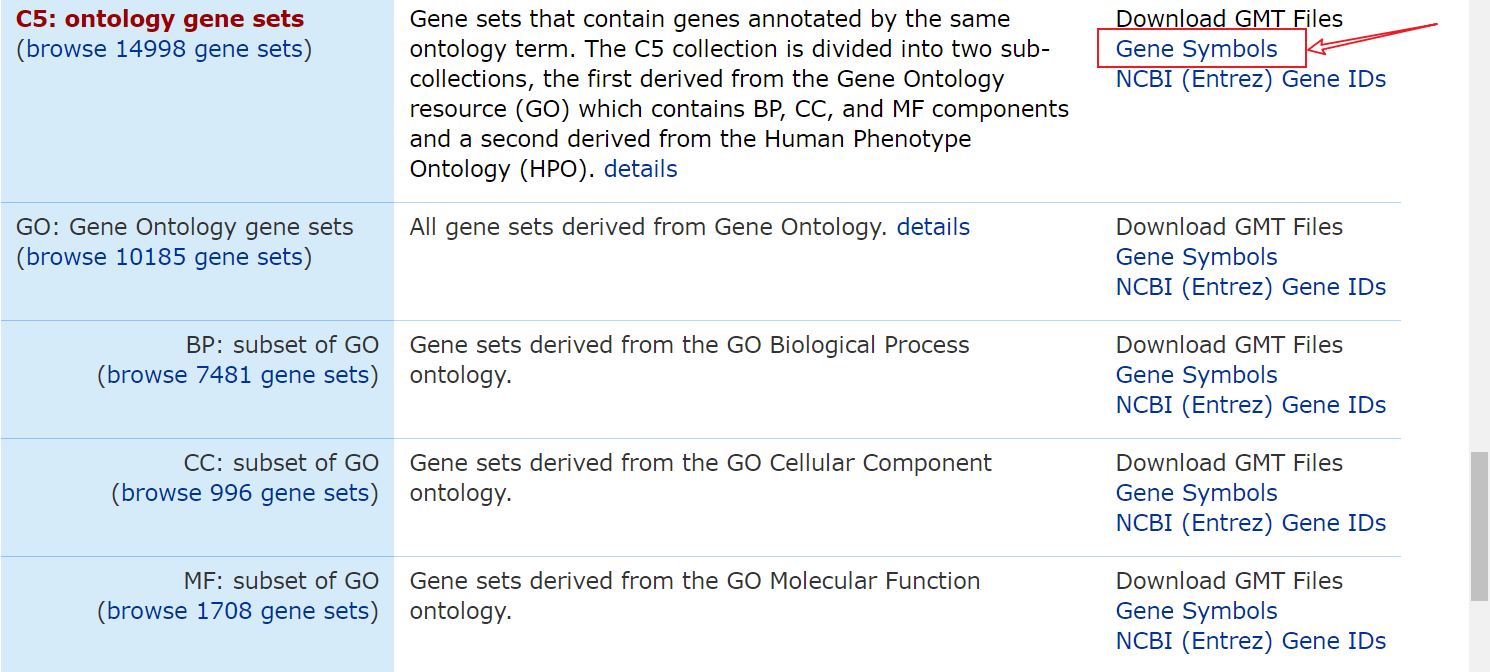
我依据分组情况,跑了其中分组为HH和LH的两组的GSEA
输入数据准备
rm(list = ls())load('Rdata/train_exp_cl.Rdata')dattrait = cl[cl$group %in% c('HL','LL'),]datexpr = exp[,rownames(dattrait)]identical(rownames(dattrait), colnames(datexpr))
DESeq2 代码同(一),命名那里我改了一下,因为不改会覆盖原来的DEG文件
DEG_DESeq2 = function(exp, group){colData <- data.frame(row.names =colnames(exp),condition=group)dds <- DESeqDataSetFromMatrix(countData = exp,colData = colData,design = ~ condition)dds <- DESeq(dds)res <- results(dds, contrast = c("condition",rev(levels(group))))resOrdered <- res[order(res$pvalue),]DEG <- as.data.frame(resOrdered)DEG = na.omit(DEG)logFC_cutoff <- with(DEG,mean(abs(log2FoldChange)) + 2*sd(abs(log2FoldChange)) )k1 = (DEG$pvalue < 0.05)&(DEG$log2FoldChange < -logFC_cutoff)k2 = (DEG$pvalue < 0.05)&(DEG$log2FoldChange > logFC_cutoff)DEG$change = ifelse(k1,"DOWN",ifelse(k2,"UP","NOT"))write.csv(DEG, file = 'outport/DEG_DESeq2_HH_LH.csv')}group = factor(dattrait$risk11, levels = c('HL','LL'))DEG_DESeq2(datexpr, group)DEG = read.csv('outport/DEG_DESeq2_HH_LH.csv')
GSEA结果处理
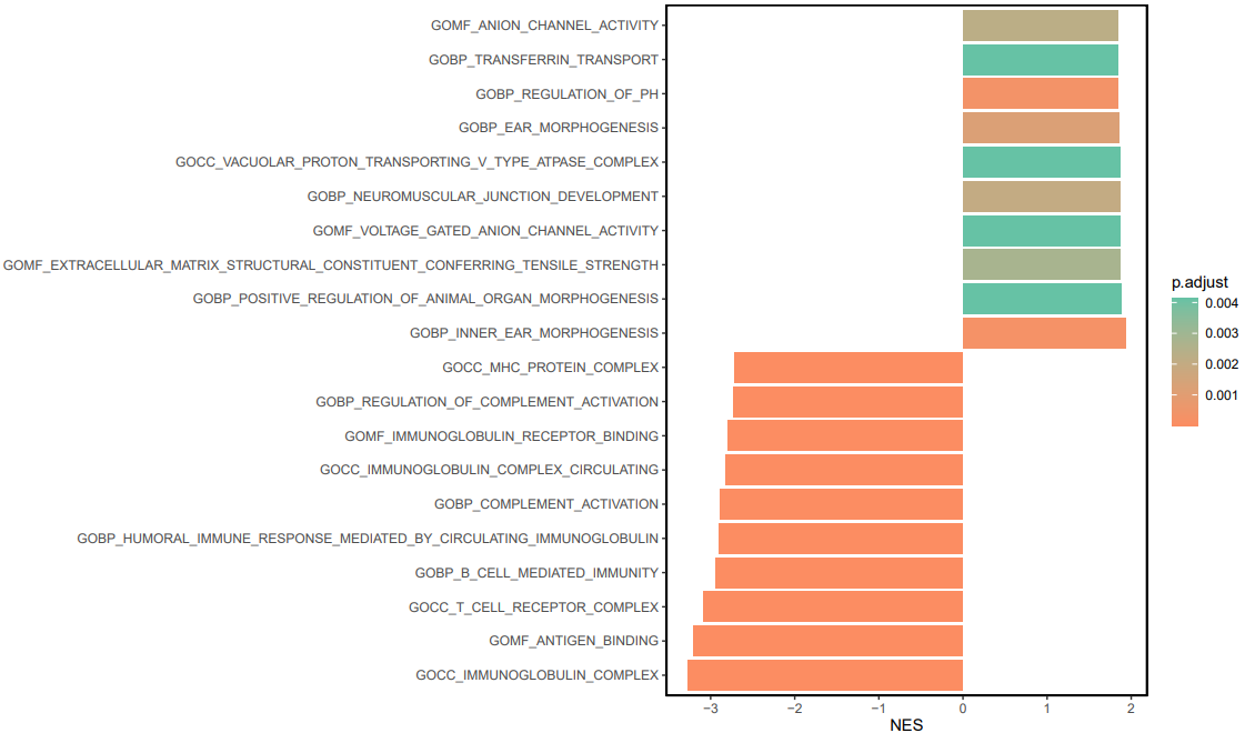
geneset = read.gmt('import/c5.go.v7.4.symbols.gmt')geneList = DEG$log2FoldChangenames(geneList) = DEG$XgeneList = sort(geneList, decreasing = T)egmt <- GSEA(geneList,TERM2GENE=geneset,verbose=T,pvalueCutoff = 1)gsea <- as.data.frame(egmt@result)gsea = gsea[gsea$p.adjust<0.01,]up = gsea[gsea$NES > 0,]dn = gsea[gsea$NES < 0,]# 太多了,就分别取了前十个作图up = up[order(up$NES, decreasing = T),]dn = dn[order(dn$NES),]x = rbind(dn[1:10,], up[1:10,])
可视化
x$Description = factor(x$Description, levels = x$Description)ggplot(x, aes(NES, Description, fill = p.adjust))+geom_barh(stat = 'identity')+scale_fill_continuous(low = "#FC8D62", high = "#66C2A5")+theme_classic()+ylab('')+theme(panel.border = element_rect(fill=NA,color="black", size=1, linetype="solid"))
成品 ↓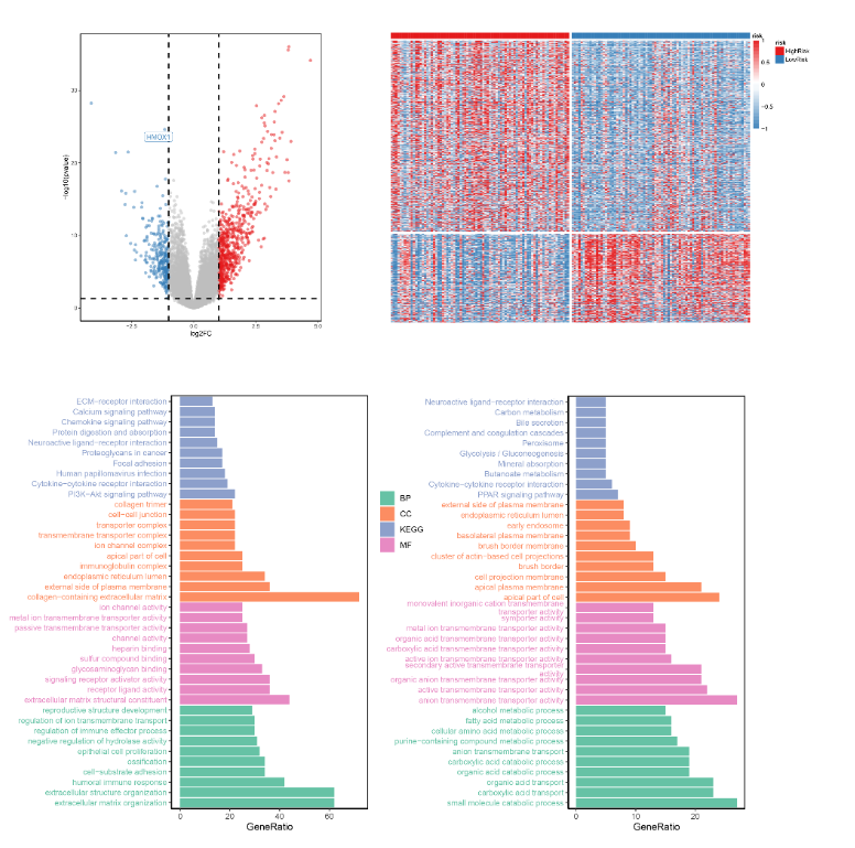

若有收获,就点个赞吧
0 人点赞
