简介
前面涉及到的都是二分类的逻辑回归问题,只要输出一个概率就可以对数据集进行二分类,但在实际生活中,对图片进行分类等
鸢尾花(iris)分类
详情
根据鸢尾花花萼和花瓣的长度和宽度对其进行分类。鸢尾属约有 300 个品种,但我们的程序将仅对下列三个品种进行分类:
- 山鸢尾
- 维吉尼亚鸢尾
- 变色鸢尾
操作步骤
1、加载IRIS数据集(训练集和验证集)
/*** @license* Copyright 2018 Google LLC. All Rights Reserved.* Licensed under the Apache License, Version 2.0 (the "License");* you may not use this file except in compliance with the License.* You may obtain a copy of the License at** http://www.apache.org/licenses/LICENSE-2.0** Unless required by applicable law or agreed to in writing, software* distributed under the License is distributed on an "AS IS" BASIS,* WITHOUT WARRANTIES OR CONDITIONS OF ANY KIND, either express or implied.* See the License for the specific language governing permissions and* limitations under the License.* =============================================================================*/import * as tf from '@tensorflow/tfjs';export const IRIS_CLASSES =['山鸢尾', '变色鸢尾', '维吉尼亚鸢尾'];export const IRIS_NUM_CLASSES = IRIS_CLASSES.length;// Iris flowers data. Source:// https://archive.ics.uci.edu/ml/machine-learning-databases/iris/iris.dataconst IRIS_DATA = [[5.1, 3.5, 1.4, 0.2, 0], [4.9, 3.0, 1.4, 0.2, 0], [4.7, 3.2, 1.3, 0.2, 0],[4.6, 3.1, 1.5, 0.2, 0], [5.0, 3.6, 1.4, 0.2, 0], [5.4, 3.9, 1.7, 0.4, 0],[4.6, 3.4, 1.4, 0.3, 0], [5.0, 3.4, 1.5, 0.2, 0], [4.4, 2.9, 1.4, 0.2, 0],[4.9, 3.1, 1.5, 0.1, 0], [5.4, 3.7, 1.5, 0.2, 0], [4.8, 3.4, 1.6, 0.2, 0],[4.8, 3.0, 1.4, 0.1, 0], [4.3, 3.0, 1.1, 0.1, 0], [5.8, 4.0, 1.2, 0.2, 0],[5.7, 4.4, 1.5, 0.4, 0], [5.4, 3.9, 1.3, 0.4, 0], [5.1, 3.5, 1.4, 0.3, 0],[5.7, 3.8, 1.7, 0.3, 0], [5.1, 3.8, 1.5, 0.3, 0], [5.4, 3.4, 1.7, 0.2, 0],[5.1, 3.7, 1.5, 0.4, 0], [4.6, 3.6, 1.0, 0.2, 0], [5.1, 3.3, 1.7, 0.5, 0],[4.8, 3.4, 1.9, 0.2, 0], [5.0, 3.0, 1.6, 0.2, 0], [5.0, 3.4, 1.6, 0.4, 0],[5.2, 3.5, 1.5, 0.2, 0], [5.2, 3.4, 1.4, 0.2, 0], [4.7, 3.2, 1.6, 0.2, 0],[4.8, 3.1, 1.6, 0.2, 0], [5.4, 3.4, 1.5, 0.4, 0], [5.2, 4.1, 1.5, 0.1, 0],[5.5, 4.2, 1.4, 0.2, 0], [4.9, 3.1, 1.5, 0.1, 0], [5.0, 3.2, 1.2, 0.2, 0],[5.5, 3.5, 1.3, 0.2, 0], [4.9, 3.1, 1.5, 0.1, 0], [4.4, 3.0, 1.3, 0.2, 0],[5.1, 3.4, 1.5, 0.2, 0], [5.0, 3.5, 1.3, 0.3, 0], [4.5, 2.3, 1.3, 0.3, 0],[4.4, 3.2, 1.3, 0.2, 0], [5.0, 3.5, 1.6, 0.6, 0], [5.1, 3.8, 1.9, 0.4, 0],[4.8, 3.0, 1.4, 0.3, 0], [5.1, 3.8, 1.6, 0.2, 0], [4.6, 3.2, 1.4, 0.2, 0],[5.3, 3.7, 1.5, 0.2, 0], [5.0, 3.3, 1.4, 0.2, 0], [7.0, 3.2, 4.7, 1.4, 1],[6.4, 3.2, 4.5, 1.5, 1], [6.9, 3.1, 4.9, 1.5, 1], [5.5, 2.3, 4.0, 1.3, 1],[6.5, 2.8, 4.6, 1.5, 1], [5.7, 2.8, 4.5, 1.3, 1], [6.3, 3.3, 4.7, 1.6, 1],[4.9, 2.4, 3.3, 1.0, 1], [6.6, 2.9, 4.6, 1.3, 1], [5.2, 2.7, 3.9, 1.4, 1],[5.0, 2.0, 3.5, 1.0, 1], [5.9, 3.0, 4.2, 1.5, 1], [6.0, 2.2, 4.0, 1.0, 1],[6.1, 2.9, 4.7, 1.4, 1], [5.6, 2.9, 3.6, 1.3, 1], [6.7, 3.1, 4.4, 1.4, 1],[5.6, 3.0, 4.5, 1.5, 1], [5.8, 2.7, 4.1, 1.0, 1], [6.2, 2.2, 4.5, 1.5, 1],[5.6, 2.5, 3.9, 1.1, 1], [5.9, 3.2, 4.8, 1.8, 1], [6.1, 2.8, 4.0, 1.3, 1],[6.3, 2.5, 4.9, 1.5, 1], [6.1, 2.8, 4.7, 1.2, 1], [6.4, 2.9, 4.3, 1.3, 1],[6.6, 3.0, 4.4, 1.4, 1], [6.8, 2.8, 4.8, 1.4, 1], [6.7, 3.0, 5.0, 1.7, 1],[6.0, 2.9, 4.5, 1.5, 1], [5.7, 2.6, 3.5, 1.0, 1], [5.5, 2.4, 3.8, 1.1, 1],[5.5, 2.4, 3.7, 1.0, 1], [5.8, 2.7, 3.9, 1.2, 1], [6.0, 2.7, 5.1, 1.6, 1],[5.4, 3.0, 4.5, 1.5, 1], [6.0, 3.4, 4.5, 1.6, 1], [6.7, 3.1, 4.7, 1.5, 1],[6.3, 2.3, 4.4, 1.3, 1], [5.6, 3.0, 4.1, 1.3, 1], [5.5, 2.5, 4.0, 1.3, 1],[5.5, 2.6, 4.4, 1.2, 1], [6.1, 3.0, 4.6, 1.4, 1], [5.8, 2.6, 4.0, 1.2, 1],[5.0, 2.3, 3.3, 1.0, 1], [5.6, 2.7, 4.2, 1.3, 1], [5.7, 3.0, 4.2, 1.2, 1],[5.7, 2.9, 4.2, 1.3, 1], [6.2, 2.9, 4.3, 1.3, 1], [5.1, 2.5, 3.0, 1.1, 1],[5.7, 2.8, 4.1, 1.3, 1], [6.3, 3.3, 6.0, 2.5, 2], [5.8, 2.7, 5.1, 1.9, 2],[7.1, 3.0, 5.9, 2.1, 2], [6.3, 2.9, 5.6, 1.8, 2], [6.5, 3.0, 5.8, 2.2, 2],[7.6, 3.0, 6.6, 2.1, 2], [4.9, 2.5, 4.5, 1.7, 2], [7.3, 2.9, 6.3, 1.8, 2],[6.7, 2.5, 5.8, 1.8, 2], [7.2, 3.6, 6.1, 2.5, 2], [6.5, 3.2, 5.1, 2.0, 2],[6.4, 2.7, 5.3, 1.9, 2], [6.8, 3.0, 5.5, 2.1, 2], [5.7, 2.5, 5.0, 2.0, 2],[5.8, 2.8, 5.1, 2.4, 2], [6.4, 3.2, 5.3, 2.3, 2], [6.5, 3.0, 5.5, 1.8, 2],[7.7, 3.8, 6.7, 2.2, 2], [7.7, 2.6, 6.9, 2.3, 2], [6.0, 2.2, 5.0, 1.5, 2],[6.9, 3.2, 5.7, 2.3, 2], [5.6, 2.8, 4.9, 2.0, 2], [7.7, 2.8, 6.7, 2.0, 2],[6.3, 2.7, 4.9, 1.8, 2], [6.7, 3.3, 5.7, 2.1, 2], [7.2, 3.2, 6.0, 1.8, 2],[6.2, 2.8, 4.8, 1.8, 2], [6.1, 3.0, 4.9, 1.8, 2], [6.4, 2.8, 5.6, 2.1, 2],[7.2, 3.0, 5.8, 1.6, 2], [7.4, 2.8, 6.1, 1.9, 2], [7.9, 3.8, 6.4, 2.0, 2],[6.4, 2.8, 5.6, 2.2, 2], [6.3, 2.8, 5.1, 1.5, 2], [6.1, 2.6, 5.6, 1.4, 2],[7.7, 3.0, 6.1, 2.3, 2], [6.3, 3.4, 5.6, 2.4, 2], [6.4, 3.1, 5.5, 1.8, 2],[6.0, 3.0, 4.8, 1.8, 2], [6.9, 3.1, 5.4, 2.1, 2], [6.7, 3.1, 5.6, 2.4, 2],[6.9, 3.1, 5.1, 2.3, 2], [5.8, 2.7, 5.1, 1.9, 2], [6.8, 3.2, 5.9, 2.3, 2],[6.7, 3.3, 5.7, 2.5, 2], [6.7, 3.0, 5.2, 2.3, 2], [6.3, 2.5, 5.0, 1.9, 2],[6.5, 3.0, 5.2, 2.0, 2], [6.2, 3.4, 5.4, 2.3, 2], [5.9, 3.0, 5.1, 1.8, 2],];/*** Convert Iris data arrays to `tf.Tensor`s.** @param data The Iris input feature data, an `Array` of `Array`s, each element* of which is assumed to be a length-4 `Array` (for petal length, petal* width, sepal length, sepal width).* @param targets An `Array` of numbers, with values from the set {0, 1, 2}:* representing the true category of the Iris flower. Assumed to have the same* array length as `data`.* @param testSplit Fraction of the data at the end to split as test data: a* number between 0 and 1.* @return A length-4 `Array`, with* - training data as `tf.Tensor` of shape [numTrainExapmles, 4].* - training one-hot labels as a `tf.Tensor` of shape [numTrainExamples, 3]* - test data as `tf.Tensor` of shape [numTestExamples, 4].* - test one-hot labels as a `tf.Tensor` of shape [numTestExamples, 3]*/function convertToTensors(data, targets, testSplit) {const numExamples = data.length;if (numExamples !== targets.length) {throw new Error('data and split have different numbers of examples');}// Randomly shuffle `data` and `targets`.const indices = [];for (let i = 0; i < numExamples; ++i) {indices.push(i);}tf.util.shuffle(indices);const shuffledData = [];const shuffledTargets = [];for (let i = 0; i < numExamples; ++i) {shuffledData.push(data[indices[i]]);shuffledTargets.push(targets[indices[i]]);}// Split the data into a training set and a tet set, based on `testSplit`.const numTestExamples = Math.round(numExamples * testSplit);const numTrainExamples = numExamples - numTestExamples;const xDims = shuffledData[0].length;// Create a 2D `tf.Tensor` to hold the feature data.const xs = tf.tensor2d(shuffledData, [numExamples, xDims]);// Create a 1D `tf.Tensor` to hold the labels, and convert the number label// from the set {0, 1, 2} into one-hot encoding (.e.g., 0 --> [1, 0, 0]).const ys = tf.oneHot(tf.tensor1d(shuffledTargets).toInt(), IRIS_NUM_CLASSES);// Split the data into training and test sets, using `slice`.const xTrain = xs.slice([0, 0], [numTrainExamples, xDims]);const xTest = xs.slice([numTrainExamples, 0], [numTestExamples, xDims]);const yTrain = ys.slice([0, 0], [numTrainExamples, IRIS_NUM_CLASSES]);const yTest = ys.slice([0, 0], [numTestExamples, IRIS_NUM_CLASSES]);return [xTrain, yTrain, xTest, yTest];}/*** Obtains Iris data, split into training and test sets.** @param testSplit Fraction of the data at the end to split as test data: a* number between 0 and 1.** @param return A length-4 `Array`, with* - training data as an `Array` of length-4 `Array` of numbers.* - training labels as an `Array` of numbers, with the same length as the* return training data above. Each element of the `Array` is from the set* {0, 1, 2}.* - test data as an `Array` of length-4 `Array` of numbers.* - test labels as an `Array` of numbers, with the same length as the* return test data above. Each element of the `Array` is from the set* {0, 1, 2}.*/export function getIrisData(testSplit) {return tf.tidy(() => {const dataByClass = [];const targetsByClass = [];for (let i = 0; i < IRIS_CLASSES.length; ++i) {dataByClass.push([]);targetsByClass.push([]);}for (const example of IRIS_DATA) {const target = example[example.length - 1];const data = example.slice(0, example.length - 1);dataByClass[target].push(data);targetsByClass[target].push(target);}const xTrains = [];const yTrains = [];const xTests = [];const yTests = [];for (let i = 0; i < IRIS_CLASSES.length; ++i) {const [xTrain, yTrain, xTest, yTest] =convertToTensors(dataByClass[i], targetsByClass[i], testSplit);xTrains.push(xTrain);yTrains.push(yTrain);xTests.push(xTest);yTests.push(yTest);}const concatAxis = 0;return [tf.concat(xTrains, concatAxis), tf.concat(yTrains, concatAxis),tf.concat(xTests, concatAxis), tf.concat(yTests, concatAxis)];});}
2、定义模型结构
3、训练模型并预测
相比之前损失函数,会增加准确度、训练时损失、训练集和验证集准确度等度量单位
见图:训练集损失/测试集损失 and 训练集准确度/测试集准确度 基本拟合,说明这是有效的训练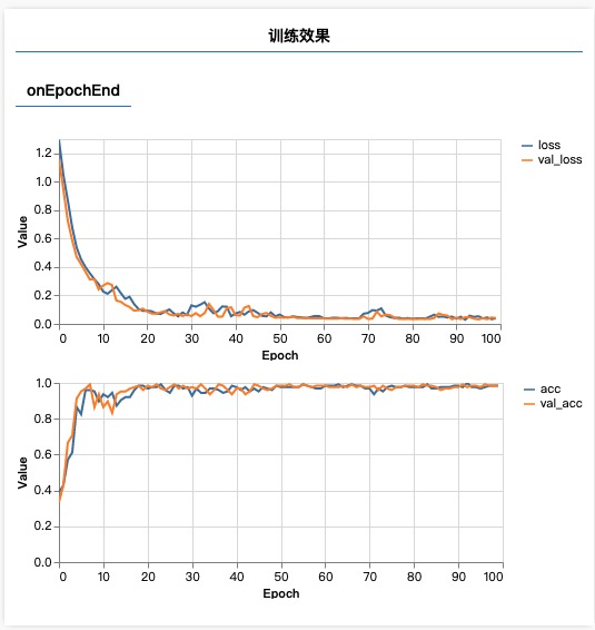
import * as tf from '@tensorflow/tfjs'import * as tfvis from '@tensorflow/tfjs-vis'import { getIrisData, IRIS_CLASSES } from './data';console.log('IRIS_CLASSES', IRIS_CLASSES)window.onload = async () => {const [xTrain, yTrain, xTest, yTest] = getIrisData(0.15);console.log('ssss', getIrisData(0.15))// 初始化模型const model = tf.sequential()model.add(tf.layers.dense({units: 10,inputShape: xTrain.shape[1] , // 或 4activation: 'sigmoid'}))model.add(tf.layers.dense({units: 3, // 因为需要输出3个概率,所以这里是3activation: 'softmax'}))// 准确度度量model.compile({loss: 'categoricalCrossentropy', // 交叉熵损失函数(解决多分类问题)optimizer: tf.train.adam(0.1),metrics: ['accuracy'] // 准确度})await model.fit(xTrain, yTrain, {epochs: 100,validationData: [xTrain, yTrain], // 验证集callbacks: tfvis.show.fitCallbacks({name: '训练效果'},['loss', 'val_loss', 'acc', 'val_acc'],{callbacks: ['onEpochEnd']})})window.predict = (form) => {const input = tf.tensor([[form.a.value * 1, // 花萼长度form.b.value * 1, // 花萼宽度form.c.value * 1, // 花瓣长度form.d.value * 1, // 花瓣宽度]]);const pred = model.predict(input); // pred.argMax(数据维度) 输出概率中的最高值alert(`预测结果:${IRIS_CLASSES[pred.argMax(1).dataSync(0)]}`);};}

若有收获,就点个赞吧
0 人点赞
