Supervised Learning

• The flowchart of Supervised Learning:

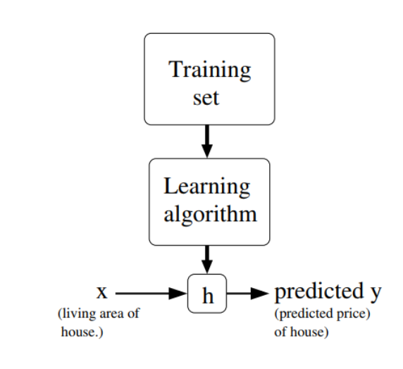
The definition of training set is as follows:

%7D%2Cy%5E%7B(i)%7D)%3Bi%20%3D%201%2C%5Ccdots%2Cn%5Cbigr%5C%7D%0A#card=math&code=%5Cbigl%5C%7B%28x%5E%7B%28i%29%7D%2Cy%5E%7B%28i%29%7D%29%3Bi%20%3D%201%2C%5Ccdots%2Cn%5Cbigr%5C%7D%0A&id=ArX0O)

By the way, the notation %7D%2Cy%7Bj%7D%5E%7B(i)%7D)#card=math&code=%5Cdisplaystyle%20%28x%7Bj%7D%5E%7B%28i%29%7D%2Cy_%7Bj%7D%5E%7B%28i%29%7D%29&id=zOK0F) means the jth features and labels of the ith training examples.

• The difference bewteen a regression problem and a classification problem.
• The goal of supervised learning is to find parameters that fit the data well.
• A example of cost function(least-squares cost function):

%3D1%2F2%5Csum%7Bi%3D1%7D%5En%7B(h%5Ctheta(x%5E%7B(i)%7D)%7D-y%5E%7B(i)%7D)%5E2%0A#card=math&code=J%28%5Ctheta%29%3D1%2F2%5Csum%7Bi%3D1%7D%5En%7B%28h%5Ctheta%28x%5E%7B%28i%29%7D%29%7D-y%5E%7B%28i%29%7D%29%5E2%0A&id=gViol)

Linear Regression

Normal Equations

For linear regression models, considering that the cost function of them just have one lowest point, they can use Normal Equations to express the proper parameters mathematically:

%5E%7B-1%7DX%5ETY%5E3%0A#card=math&code=%5Ctheta%20%3D%20%28X%5ETX%29%5E%7B-1%7DX%5ETY%5E3%0A&id=ZULV5)

Here the X and Y denotes the feature matrix and label vector respectively.

Batch Gradient Descent

The learning progress is defined as follows:

%7D)-y%5E%7B(i)%7D)x%5E%7B(i)%7D%0A#card=math&code=%5Ctheta%20%3A%3D%20%5Ctheta%20-%20%5Calpha%5Csum%7Bi%3D1%7D%5En%28h%5Ctheta%28x%5E%7B%28i%29%7D%29-y%5E%7B%28i%29%7D%29x%5E%7B%28i%29%7D%0A&id=LfUju)

• If predicted value is equal to the label, then parameters remain the same
• If predicted value is larger than the label, that means the theta is too high, then parameters goes down
• If predicted value is smaller than the label, that means the theta is too low, then parameters goes up

By the way the alpha denotes “learning rate”,which is set to 0.01 empirically.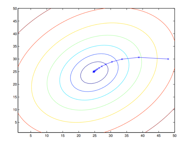

Stochastic Gradient Descent

%7D)-y%5E%7B(i)%7D)x%5E%7B(i)%7D%0A#card=math&code=%5Ctheta%20%3A%3D%20%5Ctheta%20-%20%5Calpha%28h_%5Ctheta%28x%5E%7B%28i%29%7D%29-y%5E%7B%28i%29%7D%29x%5E%7B%28i%29%7D%0A&id=Tb3tL)

Compared to Batch Gradient Descent, the theta is also influenced by only one training example in Stochastic Gradient Descent. That’s the reason why it is called ‘Stochastic’. So the advantage of Stochastic Gradient Descent is that when the dataset is large, using Stochastic Gradient Descent instead of Batch Gradient Descent saves much time.

Mini-batch Gradient Descent

It is just the combination of Stochastic Gradient Descent and Batch Gradient Descent, the training progress of it is just as follows:

1. Devide the large dataset into mant batches
2. each loop use a batch of them to update the parameter
3. Repeart 1 and 2

So Mini-batch Gradient Descent is a trade-off between convergence and training speed.

Probabilistic interpretation

The detailed interpretation can be seen in the lecture notes1, the core interpretation is as follows:

%7D%20%3D%20%5Ctheta%5ETx%5E%7B(i)%7D%2B%5Cepsilon%5E%7B(i)%7D%0A#card=math&code=y%5E%7B%28i%29%7D%20%3D%20%5Ctheta%5ETx%5E%7B%28i%29%7D%2B%5Cepsilon%5E%7B%28i%29%7D%0A&id=xck6M)

the error satisfies:

%7D)%20%3D%20%5Cfrac%7B1%7D%7B(2%5Cpi)%5E%7B0.5%7D%5Csigma%7Dexp(-%5Cfrac%7B(%5Cepsilon%5E%7B(i)%7D)%5E2%7D%7B2%5Csigma%5E2%7D)%0A#card=math&code=p%28%5Cepsilon%5E%7B%28i%29%7D%29%20%3D%20%5Cfrac%7B1%7D%7B%282%5Cpi%29%5E%7B0.5%7D%5Csigma%7Dexp%28-%5Cfrac%7B%28%5Cepsilon%5E%7B%28i%29%7D%29%5E2%7D%7B2%5Csigma%5E2%7D%29%0A&id=ue7iE)

so it implies:

%7D%7Cx%5E%7B(i)%7D%3B%5Ctheta)%20%3D%20%5Cfrac%7B1%7D%7B(2%5Cpi)%5E%7B0.5%7D%5Csigma%7Dexp(-%5Cfrac%7B(y%5E%7B(i)%7D-%5Ctheta%5ETx%5E%7B(i)%7D)%5E2%7D%7B2%5Csigma%5E2%7D)%0A#card=math&code=p%28y%5E%7B%28i%29%7D%7Cx%5E%7B%28i%29%7D%3B%5Ctheta%29%20%3D%20%5Cfrac%7B1%7D%7B%282%5Cpi%29%5E%7B0.5%7D%5Csigma%7Dexp%28-%5Cfrac%7B%28y%5E%7B%28i%29%7D-%5Ctheta%5ETx%5E%7B%28i%29%7D%29%5E2%7D%7B2%5Csigma%5E2%7D%29%0A&id=ViXJV)

log maximum likelihood function can be written as:

%3D%5Csum%7Bi%3D1%7D%5Enlog%5Cbigl%5C%7B%5Cfrac%7B1%7D%7B(2%5Cpi)%5E%7B0.5%7D%5Csigma%7Dexp(-%5Cfrac%7B(y%5E%7B(i)%7D-%5Ctheta%5ETx%5E%7B(i)%7D)%5E2%7D%7B2%5Csigma%5E2%7D)%5Cbigr%5C%7D%0A#card=math&code=L%28%5Ctheta%29%3D%5Csum%7Bi%3D1%7D%5Enlog%5Cbigl%5C%7B%5Cfrac%7B1%7D%7B%282%5Cpi%29%5E%7B0.5%7D%5Csigma%7Dexp%28-%5Cfrac%7B%28y%5E%7B%28i%29%7D-%5Ctheta%5ETx%5E%7B%28i%29%7D%29%5E2%7D%7B2%5Csigma%5E2%7D%29%5Cbigr%5C%7D%0A&id=TOoOw)

Hence, maximizing $ L(\theta)$gives the same answer as minimizing :

%7D-%5Ctheta%5ETx%5E%7B(i)%7D)%5E2%0A#card=math&code=1%2F2%5Csum_%7Bi%3D1%7D%5En%28y%5E%7B%28i%29%7D-%5Ctheta%5ETx%5E%7B%28i%29%7D%29%5E2%0A&id=Dw3Bq)

which we recognize to be #card=math&code=J%28%5Ctheta%29&id=FiKEL), our original least-squares cost function.

Locally Weighted Linear Regression

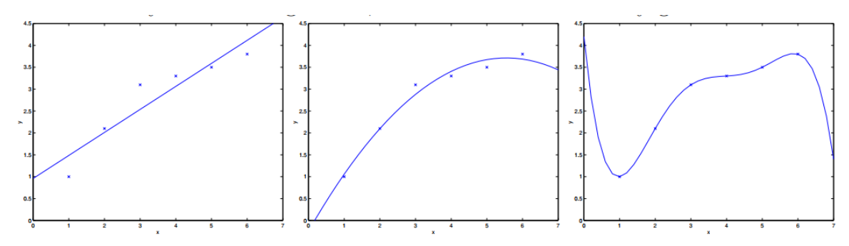
The leftmost picture is underfitting while the rightmost picture is overfitting, which are neither good.

• The difference between non-parametric algorithm and parametric algorithm

  Classification and Logistic Regression

  In a classification problem, we often refer to a binary classification in which there are just two classes.

  Logistic Regression

  We will choose:

%20%3D%20g(%5Ctheta%5ETX)%3D%5Cfrac%7B1%7D%7B1%2Be%5E%7B-%5Ctheta%5ETX%7D%7D%0A#card=math&code=h_%5Ctheta%28x%29%20%3D%20g%28%5Ctheta%5ETX%29%3D%5Cfrac%7B1%7D%7B1%2Be%5E%7B-%5Ctheta%5ETX%7D%7D%0A&id=U3Rjs)

is called logistic function, its curve is like:

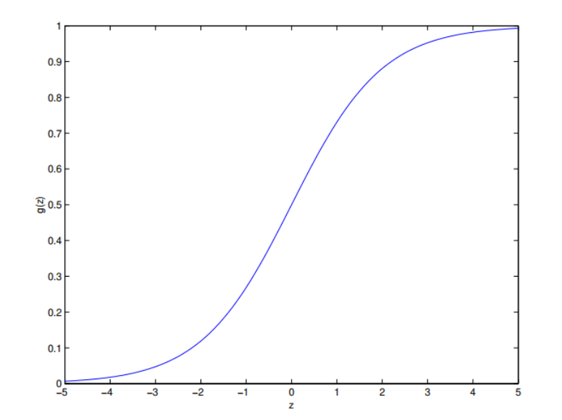
here’s a useful property of the derivative of the sigmoid function:

%20%3D%20g(z)(1-g(z))%0A#card=math&code=g%27%28z%29%20%3D%20g%28z%29%281-g%28z%29%29%0A&id=jFSJC)

The fact that many specific functions are chosen in machine learning is bacause they have some good properties that are conducive to computational efficiency.
For Logistic Regression and binary classification, it is:

%3D(h%5Ctheta(x))%5Ey(1-h%5Ctheta(x))%5E%7B1-y%7D%0A#card=math&code=p%28y%7Cx%3B%5Ctheta%29%3D%28h%5Ctheta%28x%29%29%5Ey%281-h%5Ctheta%28x%29%29%5E%7B1-y%7D%0A&id=HoWI1)

maximum log likelihood:

%3D%5Csum%7Bi%3D1%7D%5Eny%5E%7B(i)%7Dlogh%5Ctheta(x%5E%7B(i)%7D)%2B(1-y%5E%7B(i)%7D)log(1-h%5Ctheta(x%5E%7B(i)%7D))%0A#card=math&code=L%28%5Ctheta%29%3D%5Csum%7Bi%3D1%7D%5Eny%5E%7B%28i%29%7Dlogh%5Ctheta%28x%5E%7B%28i%29%7D%29%2B%281-y%5E%7B%28i%29%7D%29log%281-h%5Ctheta%28x%5E%7B%28i%29%7D%29%29%0A&id=IoU4y)

For this, we use the stochastic gradient ascent rule to train the model:

%7D-h%5Ctheta(x%5E%7B(i)%7D))x%5E%7B(i)%7D%0A#card=math&code=%5Ctheta_j%20%3A%3D%5Ctheta_j%20%2B%20%5Calpha%28y%5E%7B%28i%29%7D-h%5Ctheta%28x%5E%7B%28i%29%7D%29%29x%5E%7B%28i%29%7D%0A&id=HwrYr)

But now the is a non-linear function.

Digression

The can be also defined as:

%20%3D%20%5Cleft%5C%7B%0A%5Cbegin%7Barray%7D%7Brl%7D%0A1%20%26%20%5Ctext%7Bif%20%7D%20z%20%3E%3D%200%2C%5C%5C%0A0%20%26%20%5Ctext%7Bif%20%7D%20z%20%3C%200%2C%5C%5C%0A%5Cend%7Barray%7D%20%5Cright.%0A#card=math&code=g%28z%29%20%3D%20%5Cleft%5C%7B%0A%5Cbegin%7Barray%7D%7Brl%7D%0A1%20%26%20%5Ctext%7Bif%20%7D%20z%20%3E%3D%200%2C%5C%5C%0A0%20%26%20%5Ctext%7Bif%20%7D%20z%20%3C%200%2C%5C%5C%0A%5Cend%7Barray%7D%20%5Cright.%0A&id=fpVgK)

then we have the perceptron learning algorithm.

Newton’s Method

Here’s a picture of the Newton’s method in action: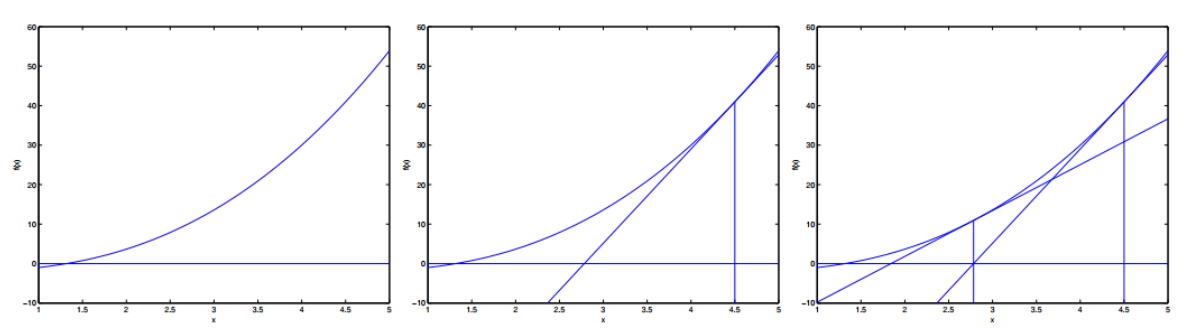

The update rule can be expressed as follows:

%7D%7BL’’(%5Ctheta)%7D%0A#card=math&code=%5Ctheta%20%3A%3D%20%5Ctheta%20-%20%5Cfrac%7BL%27%28%5Ctheta%29%7D%7BL%27%27%28%5Ctheta%29%7D%0A&id=cPHqu)

Then for training, our parameters are vectorized, so the rule can be changed as follows:

where is called Hessian Matrix.

Generalized Linear Models

The Exponential Family

We say that a class of distributions is in the exponential family if it can be written in the form:

%3Db(y)exp(%5Ceta%5ETT(y)-a(%5Ceta))%0A#card=math&code=p%28y%3B%5Ceta%29%3Db%28y%29exp%28%5Ceta%5ETT%28y%29-a%28%5Ceta%29%29%0A&id=v9Dyj)

By changing these functions, we can get Bernoulli, Gaussian and so on.

Constructing GLMs

There are three important assumptions about Generalized Linear Models:

1. given and , the distribution of follows some exponential family distribution, with parameter
2. The output of GLM(hypothesis) is the expectation of the model
3. 

So Generalized Linear Models are built as follows:

1. 
2. Use The Exponential Family to make it a non-linear model
3. Train it

   Generative Learning Algorithms

• The difference between discriminative learning algorithms and generative learning algorithms

discriminative learning algorithms: Algorithms that try to learn directly
generative learning algorithms: Algorithms that try to learn (class priors)and
because of bayesian rule:

%20%3D%20%5Cfrac%7Bp(y)p(x%7Cy)%7D%7Bp(x)%7D%0A#card=math&code=p%28y%7Cx%29%20%3D%20%5Cfrac%7Bp%28y%29p%28x%7Cy%29%7D%7Bp%28x%29%7D%0A&id=qBFdX)

Actually, if were calculating #card=math&code=p%28y%7Cx%29&id=SfYtV) in order to make a prediction, then we don’t actually need to calculate
the denominator, since we need to calculate .

Gaussian Discriminant Analysis

Multivariate Normal Distribution

its density is given by:

%20%3D%20%5Cfrac%7B1%7D%7B(2%5Cpi)%5E%7Bd%2F2%7D%7C%5Csigma%7C%5E%7B1%2F2%7D%7Dexp(-%5Cfrac%7B1%7D%7B2%7D(x-%5Cmu)%5ET%5Csigma%5E%7B-1%7D(x-%5Cmu))%0A#card=math&code=p%28x%7C%5Cmu%3B%5Csigma%29%20%3D%20%5Cfrac%7B1%7D%7B%282%5Cpi%29%5E%7Bd%2F2%7D%7C%5Csigma%7C%5E%7B1%2F2%7D%7Dexp%28-%5Cfrac%7B1%7D%7B2%7D%28x-%5Cmu%29%5ET%5Csigma%5E%7B-1%7D%28x-%5Cmu%29%29%0A&id=mv9ud)

%3D%5Csigma%0A#card=math&code=Cov%28X%29%3D%5Csigma%0A&id=zLUGv)

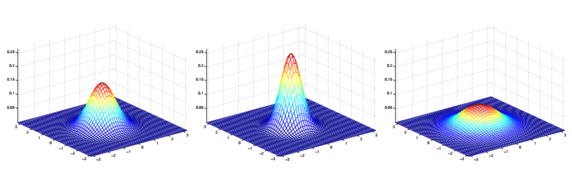
The curve or hyperplane is more steep, then the is smaller. And the center is exactly the same as

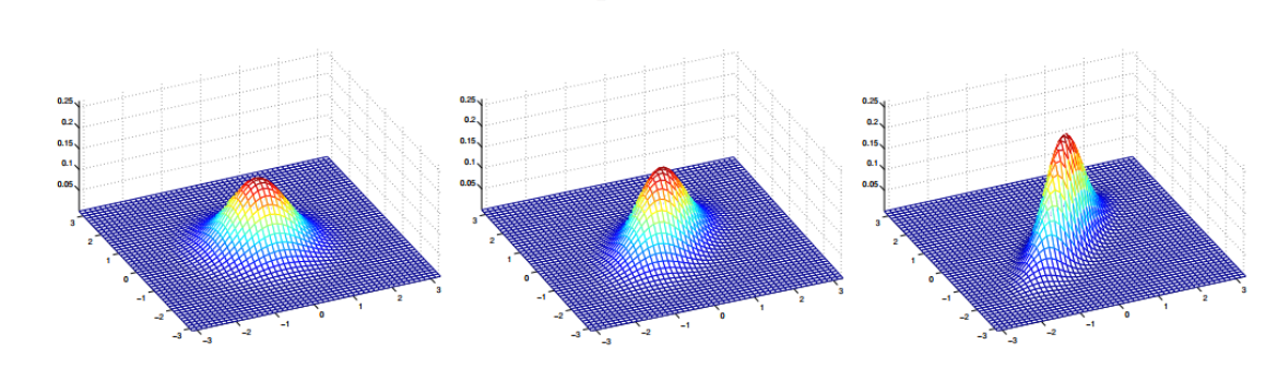
Then if is not a dialog matrix, it implies that the two dimensions shows a correlation.

Gaussian Discriminant Analysis Model

There are three formulas showing the GDA model:

%20%3D%20%5Cphi%5Ey(1-%5Cphi)%5E%7B(1-y)%7D%0A#card=math&code=p%28y%29%20%3D%20%5Cphi%5Ey%281-%5Cphi%29%5E%7B%281-y%29%7D%0A&id=vgwbx)

%3D%5Cfrac%7B1%7D%7B(2%5Cpi)%5E%7Bd%2F2%7D%7C%5Csigma%7C%5E%7B1%2F2%7D%7Dexp(-%5Cfrac%7B1%7D%7B2%7D(x-%5Cmu_0)%5ET%5Csigma%5E%7B-1%7D(x-%5Cmu_0))%0A#card=math&code=p%28x%7Cy%3D0%29%3D%5Cfrac%7B1%7D%7B%282%5Cpi%29%5E%7Bd%2F2%7D%7C%5Csigma%7C%5E%7B1%2F2%7D%7Dexp%28-%5Cfrac%7B1%7D%7B2%7D%28x-%5Cmu_0%29%5ET%5Csigma%5E%7B-1%7D%28x-%5Cmu_0%29%29%0A&id=B03CP)

%3D%5Cfrac%7B1%7D%7B(2%5Cpi)%5E%7Bd%2F2%7D%7C%5Csigma%7C%5E%7B1%2F2%7D%7Dexp(-%5Cfrac%7B1%7D%7B2%7D(x-%5Cmu_1)%5ET%5Csigma%5E%7B-1%7D(x-%5Cmu_1))%0A#card=math&code=p%28x%7Cy%3D1%29%3D%5Cfrac%7B1%7D%7B%282%5Cpi%29%5E%7Bd%2F2%7D%7C%5Csigma%7C%5E%7B1%2F2%7D%7Dexp%28-%5Cfrac%7B1%7D%7B2%7D%28x-%5Cmu_1%29%5ET%5Csigma%5E%7B-1%7D%28x-%5Cmu_1%29%29%0A&id=YdBW5)

These three formulas mean that:

1. y satisfies Bernoulli
2. two classes satisfies Gaussion Multivariate Normal Distribution respectively

By maximizing log-likelihood with respect to the parameters, we find the maximum likelihood estimate of the parameters (see problem set 1) to be:

%7D%3D1)%0A#card=math&code=%5Cphi%20%3D%20%5Cfrac%7B1%7D%7Bn%7D%5Csum_%7Bi%3D1%7D%5EnI%28y%5E%7B%28i%29%7D%3D1%29%0A&id=dvHjA)

%7D%3D0)x%5E%7B(i)%7D%7D%7B%5Csum%7Bi%3D1%7D%5EnI(y%5E%7B(i)%7D%3D0)%7D%0A#card=math&code=%5Cmu_0%20%3D%20%5Cfrac%7B%5Csum%7Bi%3D1%7D%5EnI%28y%5E%7B%28i%29%7D%3D0%29x%5E%7B%28i%29%7D%7D%7B%5Csum_%7Bi%3D1%7D%5EnI%28y%5E%7B%28i%29%7D%3D0%29%7D%0A&id=u3KoK)

%7D%3D1)x%5E%7B(i)%7D%7D%7B%5Csum%7Bi%3D1%7D%5EnI(y%5E%7B(i)%7D%3D1)%7D%0A#card=math&code=%5Cmu_1%20%3D%20%5Cfrac%7B%5Csum%7Bi%3D1%7D%5EnI%28y%5E%7B%28i%29%7D%3D1%29x%5E%7B%28i%29%7D%7D%7B%5Csum_%7Bi%3D1%7D%5EnI%28y%5E%7B%28i%29%7D%3D1%29%7D%0A&id=zTbsH)

%7D-%5Cmu%7By%5E%7B(i)%7D%7D)(x%5E%7B(i)%7D-%5Cmu%7By%5E%7B(i)%7D%7D)%5ET%0A#card=math&code=%5Csigma%20%3D%20%5Cfrac%7B1%7D%7Bn%7D%5Csum%7Bi%3D1%7D%5En%28x%5E%7B%28i%29%7D-%5Cmu%7By%5E%7B%28i%29%7D%7D%29%28x%5E%7B%28i%29%7D-%5Cmu_%7By%5E%7B%28i%29%7D%7D%29%5ET%0A&id=t2fNo)

Pictorially, what the algorithm is doing can be seen in as follows: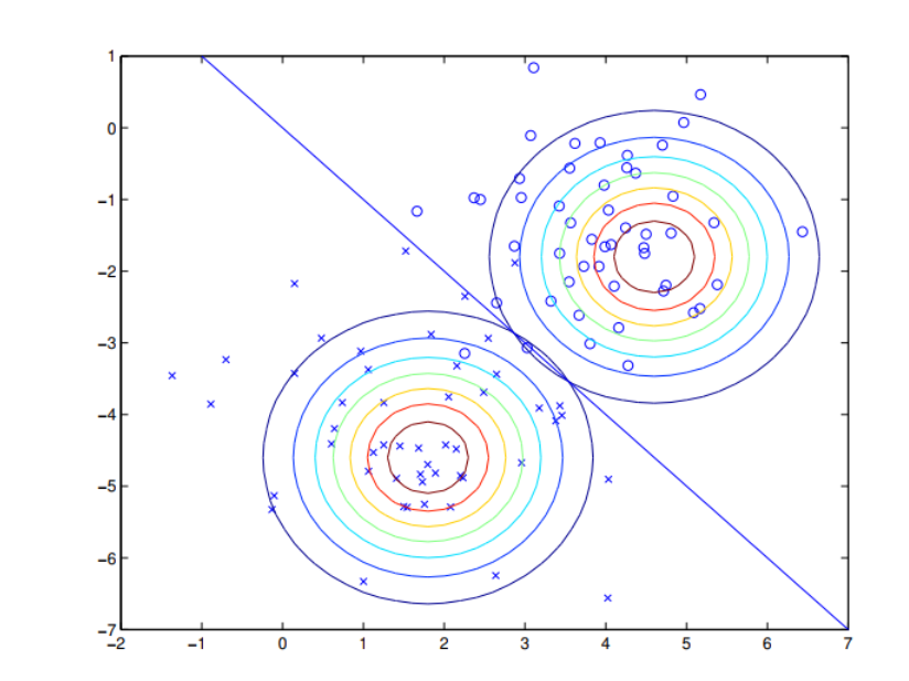

Naive Bayes

Naive bayes is similer to GDA model except for discretevalued features.
We will therefore make a very strong assumption:
We will assume that the ’s are conditionally independent given .
so:

%20%3D%20p(x%7Cy)p(y)%20%3D%20p(y)%5Cprod%7Bj%3D1%7D%5Edp(x_j%7Cy)%0A#card=math&code=p%28y%7Cx%29%20%3D%20p%28x%7Cy%29p%28y%29%20%3D%20p%28y%29%5Cprod%7Bj%3D1%7D%5Edp%28x_j%7Cy%29%0A&id=Dw4hN)

For a binary classification problem:
%20%3D%20p(x%7Cy%3D0)p(y%3D0)%20%3D%20p(y)%5Cprod%7Bj%3D1%7D%5Edp(x_j%7Cy%3D0)%0A#card=math&code=p%28y%3D0%7Cx%29%20%3D%20p%28x%7Cy%3D0%29p%28y%3D0%29%20%3D%20p%28y%29%5Cprod%7Bj%3D1%7D%5Edp%28xj%7Cy%3D0%29%0A&id=ao8NI)
%20%3D%20p(x%7Cy%3D1)p(y%3D1)%20%3D%20p(y)%5Cprod%7Bj%3D1%7D%5Edp(xj%7Cy%3D1)%0A#card=math&code=p%28y%3D1%7Cx%29%20%3D%20p%28x%7Cy%3D1%29p%28y%3D1%29%20%3D%20p%28y%29%5Cprod%7Bj%3D1%7D%5Edp%28x_j%7Cy%3D1%29%0A&id=fysd3)
There are two main advantages of it:

1. We note that even though the Naive Bayes assumption is an extremely strong assumptions, the resulting algorithm works well on many problems.
2. Naive Bayes does not need loop for optimization, so it runs fast but it is also dirty

And if the question given to us is not discretevalued, we can discretize it then use Naive Bayes.

Laplace Smoothing

The Naive Bayes algorithm as we have described it will work fairly well for many problems, but there is a simple change that makes it work much better, especially for text classification.
for , if we have not seen x yet, then p(x) will be zero.
If we have k features in x, then the formula can be written as:

%3D%5Cfrac%7B1%2B%5Csum%7Bi%3D1%7D%5EnI(z%5E%7B(i)%7D%3Dj)%7D%7Bk%2Bn%7D%0A#card=math&code=%5Cphi_j%3Dp%28z%3Dj%29%3D%5Cfrac%7B1%2B%5Csum%7Bi%3D1%7D%5EnI%28z%5E%7B%28i%29%7D%3Dj%29%7D%7Bk%2Bn%7D%0A&id=Gutib)

Event Models for Text Classification

See the lecture notes.

Kernel Methods

We start by considering fitting cubic functions

%0A#card=math&code=%5Ctheta_3x%5E3%2B%5Ctheta_2x%5E2%2B%5Ctheta_1x%5E%2B%5Ctheta_0%3D%5Ctheta%5ET%5Cphi%28x%29%0A&id=zHPgb)

Thus, a cubic function of the variable can be viewed as a linear function over the variables

• we will call the “original” input value the input attributes of a problem
• When the original input is mapped to some new set of quantities #card=math&code=%5Cphi%28x%29&id=bykv6), we will call those new quantities the features variables

  LMS with features

  To obtain the new update of batch gradient descent:

%7D)-y%5E%7B(i)%7D)%5Cphi(x%5E%7B(i)%7D)%0A#card=math&code=%5Ctheta%20%3A%3D%20%5Ctheta%20-%20%5Calpha%5Csum_%7Bi%3D1%7D%5En%28%5Ctheta%5ET%5Cphi%28x%5E%7B%28i%29%7D%29-y%5E%7B%28i%29%7D%29%5Cphi%28x%5E%7B%28i%29%7D%29%0A&id=ETMHx)

Similarly, the corresponding stochastic gradient descent update rule is:

%7D)-y%5E%7B(i)%7D)%5Cphi(x%5E%7B(i)%7D)%0A#card=math&code=%5Ctheta%20%3A%3D%20%5Ctheta%20-%20%5Calpha%28%5Ctheta%5ET%5Cphi%28x%5E%7B%28i%29%7D%29-y%5E%7B%28i%29%7D%29%5Cphi%28x%5E%7B%28i%29%7D%29%0A&id=Sxpi5)

LMS with the kernel trick

Assume at some point, can be represented as:

%3D%5Cleft%5B%20%5Cbegin%7Bmatrix%7D%201%20%5C%5C%20x_1%20%5C%5C%20x_2%20%5C%5C%20%5Ccdots%20%5C%5C%20x_1%5E2%20%5C%5C%20%5Ccdots%20%5C%5C%20x_1x_2%20%5C%5C%20%5Ccdots%20%5C%5C%20x_1%5E3%20%5C%5C%20%5Ccdots%20%5Cend%7Bmatrix%7D%20%5Cright%5D%0A#card=math&code=%5Cphi%28x%29%3D%5Cleft%5B%20%5Cbegin%7Bmatrix%7D%201%20%5C%5C%20x_1%20%5C%5C%20x_2%20%5C%5C%20%5Ccdots%20%5C%5C%20x_1%5E2%20%5C%5C%20%5Ccdots%20%5C%5C%20x_1x_2%20%5C%5C%20%5Ccdots%20%5C%5C%20x_1%5E3%20%5C%5C%20%5Ccdots%20%5Cend%7Bmatrix%7D%20%5Cright%5D%0A&id=remcb)

%7D)%0A#card=math&code=%5Ctheta%20%3D%20%5Csum_%7Bi%3D1%7D%5En%5Cbeta_i%5Cphi%28x%5E%7B%28i%29%7D%29%0A&id=XYyFP)

The rule of batch gradient descent can be replaced by:

%7D-%5Csum%7Bj%3D1%7D%5En%5Cbeta_j%5Cphi(x%5E%7B(j)%7D)%5ET%5Cphi(x%5E%7B(j)%7D))%0A#card=math&code=%5Cbeta_i%3A%3D%5Cbeta_i%20%2B%20%5Calpha%28y%5E%7B%28i%29%7D-%5Csum%7Bj%3D1%7D%5En%5Cbeta_j%5Cphi%28x%5E%7B%28j%29%7D%29%5ET%5Cphi%28x%5E%7B%28j%29%7D%29%29%0A&id=vMLpo)

wo important properties come to rescue:

1. We can pre-compute the pairwise inner products before the loop starts.
2. For the feature map, computing inner product can be effecient.

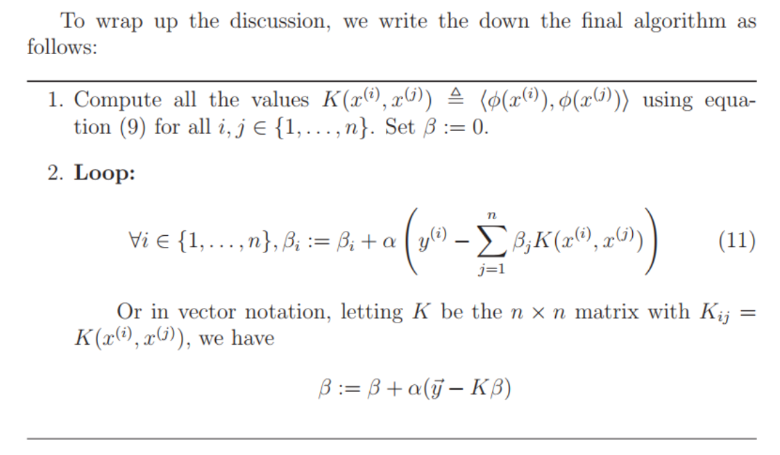
With the algorithm above, we can update the representation of the vector efficiently with O(n) time per update.

Properties of kernels

Content about this topic can be seen in the lecture notes.

Support Vector Machines

Notation

%3Dg(%5Comega%5ETx%2Bb)%0A#card=math&code=h_%7Bw%2Cb%7D%28x%29%3Dg%28%5Comega%5ETx%2Bb%29%0A&id=FIBm3)

Here, , and otherwise.

Functional and Geometric Margins

we define the functional margin of (w, b) with respect to the training example as:

%7D%3Dy%5E%7B(i)%7D(%5Comega%5ETx%5E%7B(i)%7D%2Bb)%0A#card=math&code=%5Cgamma%5E%7B%28i%29%7D%3Dy%5E%7B%28i%29%7D%28%5Comega%5ETx%5E%7B%28i%29%7D%2Bb%29%0A&id=sAxi2)

• If it is more than 0, then our prediction on this example is correct.
• Hence, a large functional margin represents a confident and a correct prediction.

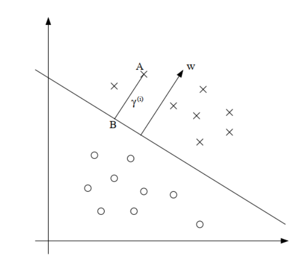
we define the geometric margin of (w, b) with respect to the training example as:

%7D%3D%5Cfrac%7By%5E%7B(i)%7D(%5Comega%5ETx%5E%7B(i)%7D%2Bb)%7D%7B%7C%7C%5Comega%7C%7C%7D%0A#card=math&code=%5Cgamma%5E%7B%28i%29%7D%3D%5Cfrac%7By%5E%7B%28i%29%7D%28%5Comega%5ETx%5E%7B%28i%29%7D%2Bb%29%7D%7B%7C%7C%5Comega%7C%7C%7D%0A&id=DPzT8)

if ||w|| = 1, then the functional margin equals the geometric margin.
Given a training set, we define the geometric margin and functional margin of the dataset as:

%7D%0A#card=math&code=%5Cgamma%20%3D%20min%20%5Cgamma%5E%7B%28i%29%7D%0A&id=qEIf0)

we now have the following optimization problem: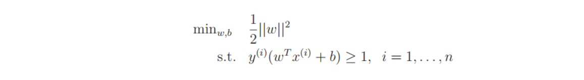

We’ve now transformed the problem into a form that can be efficiently solved. The above is an optimization problem with a convex quadratic objective and only linear constraints. Its solution gives us the optimal margin classifier. This optimization problem can be solved using commercial quadratic programming (QP) code.

Optimal Margin Classifiers

Content about this topic can be seen in the lecture notes.

Regularization and the Non-separable Case

The derivation of the SVM as presented so far assumed that the data is linearly separable.
Also, in some cases it is not clear that finding a separating hyperplane is exactly what we’d want to do, since that might be susceptible to outliers. For instance, the left figure below shows an optimal margin classifier, and when a single outlier is added in the upper-left region (right figure), it causes the decision boundary to make a dramatic swing, and the resulting classifier has a much smaller margin.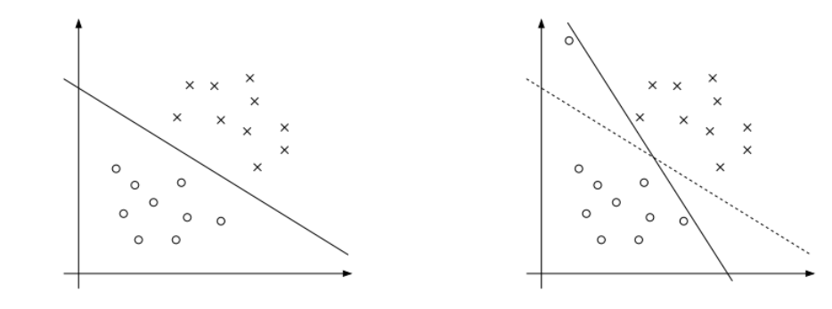

So we use L1 Regularization: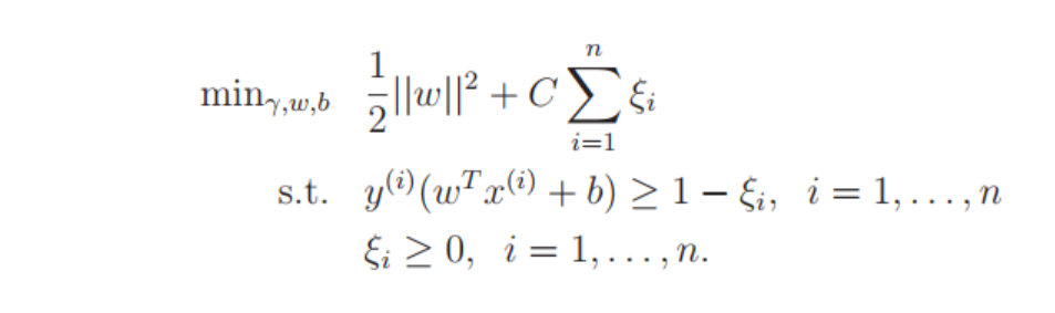

Content about this topic can be seen in the lecture notes.
The parameter C controls the relative weighting between the twin goals of making the small which we saw earlier makes the margin large and ensures that most examples have functional margin at least 1.

Regularization and Model Selection

Cross Validation

• The definition of k-fold cross validation
• A typical choice for the number of folds to use here would be k = 10

• The definition of leave-one-out cross validation

  Feature Selection

  We use the procedure called Forward search to find the best features:
  
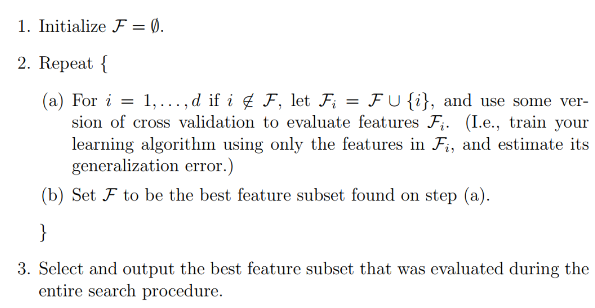
  Similarly, backward search does the opposite.
  These algorithms described above two instantiations of wrapper model feature selection.
  Wrapper feature selection algorithms often work quite well, but can be computationally expensive given how that they need to make many calls to the learning algorithm.

• The difference between Filter Wrapper feature selection and feature selection

• One possible choice of the score is about the relationship between a feature and label as:

• Mutual Information(Try to understand this):

  %3D%5Csum%7Bx_i%5Cin%5C%7B0%2C1%5C%7D%7D%5Csum%7By%5Cin%5C%7B0%2C1%5C%7D%7Dp(xi%2Cy)log%5Cfrac%7Bp(x_i%2Cy)%7D%7Bp(x_i)p(y)%7D%0A#card=math&code=MI%28x_i%2Cy%29%3D%5Csum%7Bxi%5Cin%5C%7B0%2C1%5C%7D%7D%5Csum%7By%5Cin%5C%7B0%2C1%5C%7D%7Dp%28x_i%2Cy%29log%5Cfrac%7Bp%28x_i%2Cy%29%7D%7Bp%28x_i%29p%28y%29%7D%0A&id=gEcsH)

• If and are independent, then xi is clearly very “non-informative” about y, and thus the score S(i) should be small

  Bayesian Statistics and Regularization

• This view of the as being constant-valued but unknown is taken in frequentist statistics

• This view of the as being constant-valued but unknown is taken in bayesian statistics

maximum likelihood estimation (MLE) rule:

%7D%7Cx%5E%7B(i)%7D%3B%5Ctheta)%0A#card=math&code=%5Ctheta%7BMLE%7D%3Dargmax%20%5Cprod%7Bi%3D1%7D%5Enp%28y%5E%7B%28i%29%7D%7Cx%5E%7B%28i%29%7D%3B%5Ctheta%29%0A&id=BaMu4)

This view of the as being constant-valued but unknown is taken in frequentist statistics
For the Bayesian view of the world:
posterior distribution on the parameters:

%20%26%3D%20%5Cfrac%7Bp(S%7C%5Ctheta)p(%5Ctheta)%7D%7Bp(S)%7D%5C%5C%0A%26%3D%20%5Cfrac%7B(%5Cprod%7Bi%3D1%7D%5Enp(y%5E%7B(i)%7D%7Cx%5E%7B(i)%7D%2C%5Ctheta))p(%5Ctheta)%7D%7Bp(S)%7D%20%5Cend%7Balign%7D%0A#card=math&code=%5Cbegin%7Balign%7D%20p%28%5Ctheta%7CS%29%20%26%3D%20%5Cfrac%7Bp%28S%7C%5Ctheta%29p%28%5Ctheta%29%7D%7Bp%28S%29%7D%5C%5C%0A%26%3D%20%5Cfrac%7B%28%5Cprod%7Bi%3D1%7D%5Enp%28y%5E%7B%28i%29%7D%7Cx%5E%7B%28i%29%7D%2C%5Ctheta%29%29p%28%5Ctheta%29%7D%7Bp%28S%29%7D%20%5Cend%7Balign%7D%0A&id=d4TYG)

To make a prediction on new given input:

%3D%5Cint%5Ctheta%20p(y%7Cx%2C%5Ctheta)p(%5Ctheta%7CS)d%5Ctheta%0A#card=math&code=p%28y%7Cx%2CS%29%3D%5Cint%5Ctheta%20p%28y%7Cx%2C%5Ctheta%29p%28%5Ctheta%7CS%29d%5Ctheta%0A&id=V2iB2)

The predict value is the given by:

dy%0A#card=math&code=E%5By%7Cx%2CS%5D%20%3D%20%5Cint_y%20yp%28y%7Cx%2CS%29dy%0A&id=D1cYi)

Unfortunately, in general it is computationally very difficult to compute this posterior distribution. This is because it requires taking integrals over the (usually high-dimensional) .
One way is to replace our posterior distribution for with a single point estimate:

%7D%7Cx%5E%7B(i)%7D%2C%5Ctheta)p(%5Ctheta)%0A#card=math&code=%5Ctheta%7BMAP%7D%3Dargmax%5Ctheta%5Cprod_%7Bi%3D1%7D%5Enp%28y%5E%7B%28i%29%7D%7Cx%5E%7B%28i%29%7D%2C%5Ctheta%29p%28%5Ctheta%29%0A&id=tKuLS)

Evaluation Metrics

Bias-Variance-Error

To put it in a nutshell, the goal of learning algorithm is to balance between bias and variance to gain better error performance and gain a good machine learning model.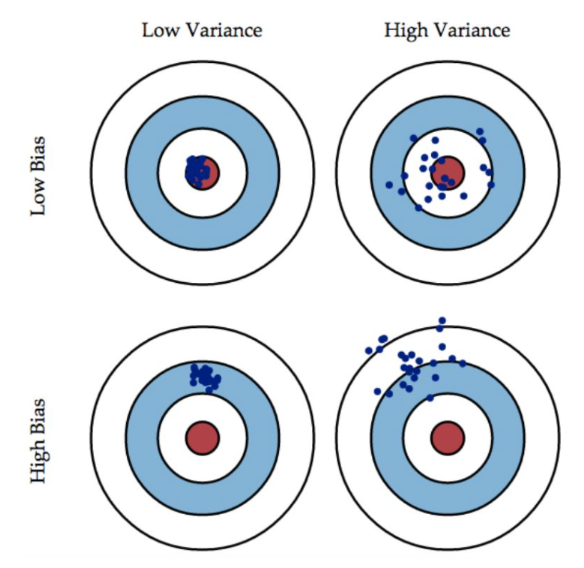

Choosing Metrics

• Confusion Matrix:

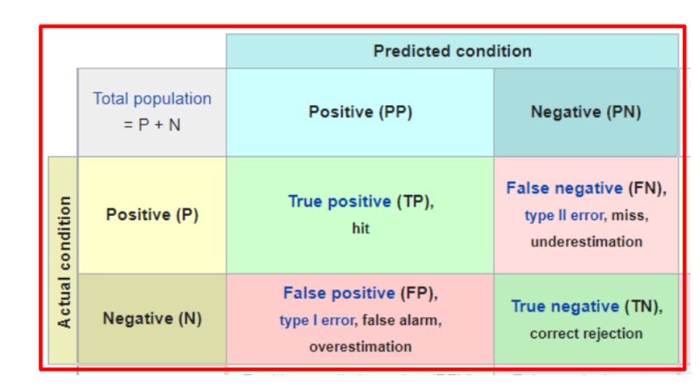
• precision\specificity\sensitivity(recall)\Accuracy\F1 Score

This picture shows everything you want to know: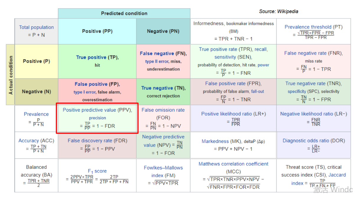

• ROC: FPR-x & TPR-y 曲线面积积分为0.5-1，越大说明模型性能越好

  Class Imbalance

• Symptom: Prevalence < 5%

• Learning: May not focus on minority class examples at all
• In general: Accuracy < AUROC < AUPRC
• We can load weights for different imbalance class

  Decision Trees

  Greedy Decision Tree Learning

  Overfitting in Decision Trees

There are two techniques processing overfitting:

1. Early Stopping

Stopping conditions (recap):

• All examples have the same target value
• No more features to split on

Early stopping conditions:

• Limit tree depth (choose max_depth using validation set)
• Do not consider splits that do not cause a sufficient decrease in classification error
• Do not split an intermediate node which contains too few data points

1. Pruning

Scoring trees：Want to balance how well the tree fits the data and the complexity of the tree
Tree pruning algorithm: Search for some information online

Ensembling Techniques

Bagging

It is also named Bootstrap Aggregating, so the procedure of bagging is as follows:

1. Use bootstraping to gain different training sets
2. Use different training sets to train many different hypothesis
3. Use these hypothesis to make an average prediction on the new given input

Let me explain this: If we use one training set from bootstrap to give one hypothesis, this hypothesis has high bias and low variance, and then we use many hypotheis to make an average prediction, which will lower the bias and the variance will go up a little. So bagging is conducive to the trade-off between bias and variance.
Application: From Decision Trees to Random Forest

Stacking

The procedure of Stacking is as follows:

1. Use bootstraping to gain different training sets
2. Use different training sets to train many different hypothesis
3. The outputs of these hypothesis can be aggregated through training instead of just on average

So Stacking can be viewed as bagging plus because it need another training, so it performs better.

Boosting

Boosting also uses Bootstrap to gain training set, the flowchart of it is as follow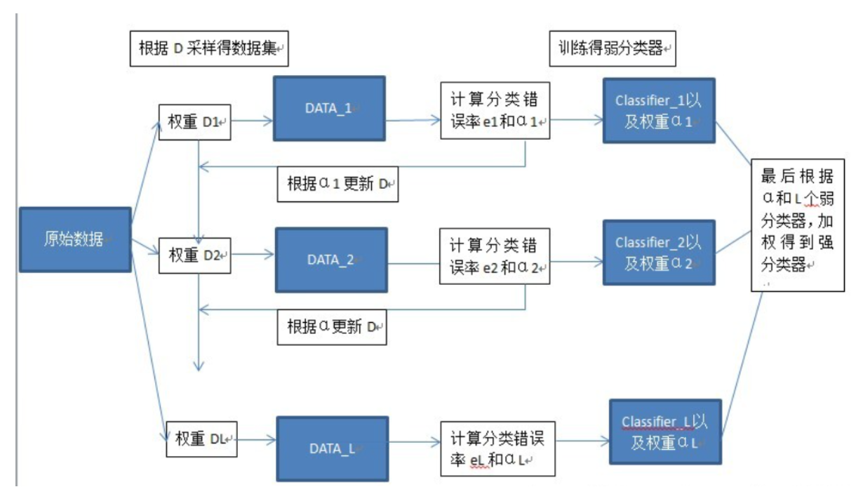

In general, it performs better then bagging and stacking because it focuses on the training examples that last classfier does not do well on.