原文:Looking at Disk Utilization and Saturation
作者:Peter Zaitsev (Percona CEO)
翻译团队:菜鸟盟
In this blog post, I will look at disk utilization and saturation.
In my previous blog post, I wrote about CPU utilization and saturation, the practical difference between them and how different CPU utilization and saturation impact response times. Now we will look at another critical component of database performance: the storage subsystem. In this post, I will refer to the storage subsystem as “disk” (as a casual catch-all).
The most common tool for command line IO performance monitoring is iostat, which shows information like this:
root@ts140i:~# iostat -x nvme0n1 5Linux 4.4.0-89-generic (ts140i) 08/05/2017 _x86_64_ (4 CPU)avg-cpu: %user %nice %system %iowait %steal %idle0.51 0.00 2.00 9.45 0.00 88.04Device: rrqm/s wrqm/s r/s w/s rkB/s wkB/s avgrq-sz avgqu-sz await r_await w_await svctm %utilnvme0n1 0.00 0.00 3555.57 5887.81 52804.15 87440.73 29.70 0.53 0.06 0.13 0.01 0.05 50.71avg-cpu: %user %nice %system %iowait %steal %idle0.60 0.00 1.06 20.77 0.00 77.57Device: rrqm/s wrqm/s r/s w/s rkB/s wkB/s avgrq-sz avgqu-sz await r_await w_await svctm %utilnvme0n1 0.00 0.00 7612.80 0.00 113507.20 0.00 29.82 0.97 0.13 0.13 0.00 0.12 93.68avg-cpu: %user %nice %system %iowait %steal %idle0.50 0.00 1.26 6.08 0.00 92.16Device: rrqm/s wrqm/s r/s w/s rkB/s wkB/s avgrq-sz avgqu-sz await r_await w_await svctm %utilnvme0n1 0.00 0.00 7653.20 0.00 113497.60 0.00 29.66 0.99 0.13 0.13 0.00 0.12 93.52
The first line shows the average performance since system start. In some cases, it is useful to compare the current load to the long term average. In this case, as it is a test system, it can be safely ignored. The next line shows the current performance metrics over five seconds intervals (as specified in the command line).
The iostat command reports utilization information in the %util column, and you can look at saturation by either looking at the average request queue size (the avgqu-sz column) or looking at the r_await and w_await columns (which show the average wait for read and write operations). If it goes well above “normal” then the device is over-saturated.
As in my previous blog post, we’ll perform some system Sysbench runs and observe how the iostat command line tool and Percona Monitoring and Management graphs behave.
To focus specifically on the disk, we’re using the Sysbench fileio test. I’m using just one 100GB file, as I’m using DirectIO so all requests hit the disk directly. I’m also using “sync” request submission mode so I can get better control of request concurrency.
I’m using an Intel 750 NVME SSD in this test (though it does not really matter).
Sysbench FileIO 1 Thread
root@ts140i:/mnt/data# sysbench --threads=1 --time=600 --max-requests=0 fileio --file-num=1 --file-total-size=100G --file-io-mode=sync --file-extra-flags=direct --file-test-mode=rndrd runFile operations:reads/s: 7113.16writes/s: 0.00fsyncs/s: 0.00Throughput:read, MiB/s: 111.14written, MiB/s: 0.00General statistics:total time: 600.0001stotal number of events: 4267910Latency (ms):min: 0.07avg: 0.14max: 6.1895th percentile: 0.17
A single thread run is always great as a baseline, as with only one request in flight we should expect the best response time possible (though typically not the best throughput possible).
IostatDevice: rrqm/s wrqm/s r/s w/s rkB/s wkB/s avgrq-sz avgqu-sz await r_await w_await svctm %utilnvme0n1 0.00 0.00 7612.80 0.00 113507.20 0.00 29.82 0.97 0.13 0.13 0.00 0.12 93.68
Disk Latency

The Disk Latency graph confirms the disk IO latency we saw in the iostat command, and it will be highly device-specific. We use it as a baseline to compare changes to with higher concurrency.
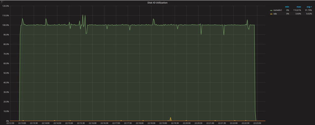
Disk IO Utilization

Disk IO utilization is close to 100% even though we have just one outstanding IO request (queue depth). This is the problem with Linux disk utilization reporting: unlike CPUs, Linux does not have direct visibility on how the IO device is designed. How many “execution units” does it really have? How are they utilized? Single spinning disks can be seen as a single execution unit while RAID, SSDs and cloud storage (such as EBS) are more than one.
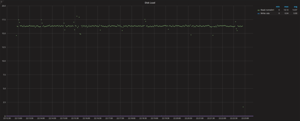
Disk Load

This graph shows the disk load (or request queue size), which roughly matches the number of threads that are hitting disk as hard as possible.
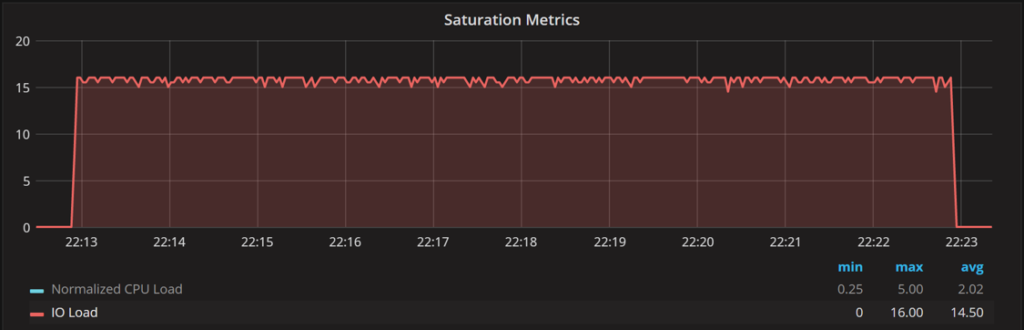
Saturation (IO Load)

The IO load on the Saturation Metrics graph shows pretty much the same numbers. The only difference is that unlike Disk IO statistics, it shows the summary for the whole system.
Sysbench FileIO 4 Threads
Now let’s increase IO to four concurrent threads and see how disk responds:
sysbench --threads=4 --time=600 --max-requests=0 fileio --file-num=1 --file-total-size=100G --file-io-mode=sync --file-extra-flags=direct --file-test-mode=rndrd runFile operations:reads/s: 26248.44writes/s: 0.00fsyncs/s: 0.00Throughput:read, MiB/s: 410.13written, MiB/s: 0.00General statistics:total time: 600.0002stotal number of events: 15749205Latency (ms):min: 0.06avg: 0.15max: 8.7395th percentile: 0.21
We can see the number of requests scales almost linearly, while request latency changes very little: 0.14ms vs. 0.15ms. This shows the device has enough execution units internally to handle the load in parallel, and there are no other bottlenecks (such as the connection interface).
IostatDevice: rrqm/s wrqm/s r/s w/s rkB/s wkB/s avgrq-sz avgqu-sz await r_await w_await svctm %utilnvme0n1 0.00 0.00 28808.60 0.00 427668.00 0.00 29.69 4.05 0.14 0.14 0.00 0.03 99.92
Disk Latency

Disk Utilization

Disk Load

Saturation Metrics (IO Load)

These stats and graphs show interesting picture: we barely see a response time increase for IO requests, while utilization inches closer to 100% (with four threads submitting requests all the time, it is hard to catch the time when the disk does not have any requests in flight). The load is near four (showing the disk has to handle four requests at the time on average).
Sysbench FileIO 16 Threads
root@ts140i:/mnt/data# sysbench --threads=16 --time=600 --max-requests=0 fileio --file-num=1 --file-total-size=100G --file-io-mode=sync --file-extra-flags=direct --file-test-mode=rndrd runFile operations:reads/s: 76845.96writes/s: 0.00fsyncs/s: 0.00Throughput:read, MiB/s: 1200.72written, MiB/s: 0.00General statistics:total time: 600.0003stotal number of events: 46107727Latency (ms):min: 0.07avg: 0.21max: 9.7295th percentile: 0.36
Going from four to 16 threads, we again see a good throughput increase with a mild response time increase. If you look at the results closely, you will notice one more interesting thing: the average response time has increased from 0.15ms to 0.21ms (which is a 40% increase), while the 95% response time has increased from 0.21ms to 0.36ms (which is 71%). I also ran a separate test measuring 99% response time, and the difference is even larger: 0.26ms vs. 0.48ms (or 84%).
This is an important observation to make: once saturation starts to happen, the variance is likely to increase and some of the requests will be disproportionately affected (beyond what the average response time shows).
IostatDevice: rrqm/s wrqm/s r/s w/s rkB/s wkB/s avgrq-sz avgqu-sz await r_await w_await svctm %utilnvme0n1 0.00 0.00 82862.20 0.00 1230567.20 0.00 29.70 16.33 0.20 0.20 0.00 0.01 100.00
Disk IO Latency

Disk IO Utilization
Disk Load
Saturation Metrics IO Load
The graphs show an expected figure: the disk load and IO load from saturation are up to about 16, and utilization remains at 100%.
One thing to notice is increased jitter in the graphs. IO utilization jumps to over 100% and disk IO load spikes to 18, when there should not be as many requests in flight. This comes from how this information is gathered. An attempt is made to sample this data every second, but with the loaded system it takes time for this process to work: sometimes when we try to get the data for a one-second interval but really get data for 1.05- or 0.95-second intervals. When the math is applied to the data, it creates the spikes and dips in the graph when there should be none. You can just ignore them if you’re looking at the big picture.
Sysbench FileIO 64 Threads
Finally, let’s run sysbench with 64 concurrent threads hitting the disk:
root@ts140i:/mnt/data# sysbench --threads=64 --time=600 --max-requests=0 fileio --file-num=1 --file-total-size=100G --file-io-mode=sync --file-extra-flags=direct --file-test-mode=rndrd runFile operations:reads/s: 127840.59writes/s: 0.00fsyncs/s: 0.00Throughput:read, MiB/s: 1997.51written, MiB/s: 0.00General statistics:total time: 600.0014stotal number of events: 76704744Latency (ms):min: 0.08avg: 0.50max: 9.3495th percentile: 1.25
We can see the average has risen from 0.21ms to 0.50 (more than two times), and 95% almost tripped from 0.36ms to 1.25ms. From a practical standpoint, we can see some saturation starting to happen, but we’re still not seeing a linear response time increase with increasing numbers of parallel operations as we have seen with CPU saturation. I guess this points to the fact that this IO device has a lot of parallel capacity inside and can process requests more effectively (even going from 16 to 64 concurrent threads).
Over the series of tests, as we increased concurrency from one to 64, we saw response times increase from 0.14ms to 0.5ms (or approximately three times). The 95% response time at this time grew from 0.17ms to 1.25ms (or about seven times). For practical purposes, this is where we see the IO device saturation start to show.
IostatDevice: rrqm/s wrqm/s r/s w/s rkB/s wkB/s avgrq-sz avgqu-sz await r_await w_await svctm %utilnvme0n1 0.00 0.00 138090.20 0.00 2049791.20 0.00 29.69 65.99 0.48 0.48 0.00 0.01 100.24
We’ll skip the rest of the graphs as they basically look the same, just with higher latency and 64 requests in flight.
Sysbench FileIO 256 Threads
root@ts140i:/mnt/data# sysbench --threads=256 --time=600 --max-requests=0 fileio --file-num=1 --file-total-size=100G --file-io-mode=sync --file-extra-flags=direct --file-test-mode=rndrd runFile operations:reads/s: 131558.79writes/s: 0.00fsyncs/s: 0.00Throughput:read, MiB/s: 2055.61written, MiB/s: 0.00General statistics:total time: 600.0026stotal number of events: 78935828Latency (ms):min: 0.10avg: 1.95max: 17.0895th percentile: 3.89
IostatDevice: rrqm/s wrqm/s r/s w/s rkB/s wkB/s avgrq-sz avgqu-sz await r_await w_await svctm %utilnvme0n1 0.00 0.00 142227.60 0.00 2112719.20 0.00 29.71 268.30 1.89 1.89 0.00 0.01 100.00
With 256 threads, finally we’re seeing the linear growth of the average response time that indicates overload and queueing to process requests. There is no easy way to tell if it is due to the IO bus saturation (we’re reading 2GB/sec here) or if it is the internal device processing ability.
As we’ve seen a less than linear increase in response time going from 16 to 64 connections, and a linear increase going from 64 to 256, we can see the “optimal” concurrency for this device: somewhere between 16 and 64 connections. This allows for peak throughput without a lot of queuing.
Before we get to the summary, I want to make an important note about this particular test. The test is a random reads test, which is a very important pattern for many database workloads, but it might not be the dominant load for your environment. You might be write-bound as well, or have mainly sequential IO access patterns (which could behave differently). For those other workloads, I hope this gives you some ideas on how to also analyze them.
Another Way to Think About Saturation
When I asked the Percona staff for feedback on this blog post by, my colleague Yves Trudeau provided another way to think about saturation: measure saturation as percent increase in the average response time compared to the single user. Like this:
Threads Avg Response Time Saturation 1 0.14 – 4 0.15 1.07x or 7% 16 0.21 1.5x or 50% 64 0.50 3.6x or 260% 256 1.95 13.9x or 1290%
Summary
We can see how understanding disk utilization and saturation is much more complicated than for the CPU:
- The Utilization metric (as reported by iostat and by PMM) is not very helpful for showing true storage utilization, as it only measures the time when there is at least one request in flight. If you had the same metric for the CPU, it would correspond to something running on at least one of the cores (not very useful for highly parallel systems).
- Unlike a CPU, Linux tools do not provide us with information about the structure of the underlying storage and how much parallel load it should be able to handle without saturation. Even more so, storage might well have different low-level resources that cause saturation. For example, it could be the network connection, SATA BUS or even the kernel IO stack for older kernels and very fast storage.
- Saturation as measured by the number of requests in flight is helpful for guessing if there might be saturation, but since we do not know how many requests the device can efficiently process concurrently, just looking the raw metric doesn’t let us determine that the device is overloaded.
- Avg Response Time is a great metric for looking at saturation, but as with the response time you can’t say what response time is good or bad for this device. You need to look at it in context and compare it to the baseline. When you’re looking at the Avg Response Time, make sure you’re looking at read request response time vs. write request response time separately, and keep the average request size in mind to ensure we are comparing apples to apples.

若有收获,就点个赞吧
0 人点赞
