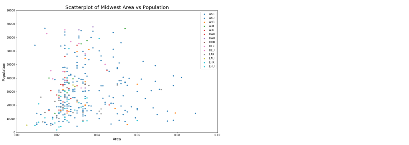
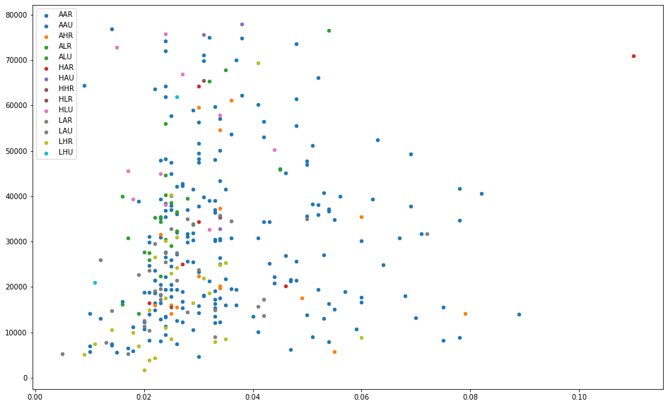
 横坐标:面积大小
总坐标:总人口
图例:暂时看不出是什么总而言之看起来是类型,一种类型一个颜色
import numpy as npimport pandas as pdimport matplotlib as mplimport matplotlib.pyplot as pltimport seaborn as sns%matplotlib inline
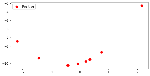
# 定义数据x1 = np.random.randn(10)x2 = x1 + x1**2 - 10# 确定画布 - 当只有一张图时不需要此步骤plt.figure(figsize = (8, 4))# 绘图plt.scatter(x1, x2 # 横坐标,纵坐标, s = 50 # 数据点尺寸大小, c = 'r' # 数据点颜色, label = 'Positive')# 装饰图形plt.legend() # 显示图例plt.show() # 显示图形
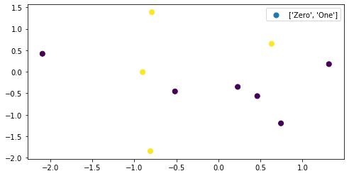
# 增加标签列yx = np.random.randn(10, 2) # 10行2列的数据集y = np.array([0, 0, 1, 1, 0, 1, 0, 1, 0, 0])plt.figure(figsize = (8, 4))plt.scatter(x[:, 0], x[:, 1], s = 50, c = y # 分类可视化, label = ['Zero', 'One'] # 无法显示理想的结果#, label = ['Zero', 'Zero', 'One', 'One', 'Zero', 'One', 'Zero', 'One', 'Zero', 'Zero'] 也无法显示理想的结果)plt.legend()
<matplotlib.legend.Legend at 0x10fc64c2710>
x[:, 0]
array([ 1.31449649, -2.09365277, -0.90142206, -0.80960202, 0.46194326,-0.79169922, 0.74378866, 0.63288047, -0.51673112, 0.22944999])
x[:, 1]
array([ 0.1774639 , 0.41847597, -0.00806844, -1.84772107, -0.56667279,1.38507805, -1.20056857, 0.65070988, -0.45736285, -0.35242212])
y
array([0, 0, 1, 1, 0, 1, 0, 1, 0, 0])
【核心知识点】可视化分类标签时的图例
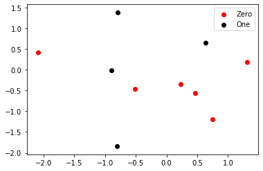
如果我们希望显示多种颜色的散点图,并且这个颜色是我们的标签y所代表的分类,那我们无法让散点图显示分别代表不同颜色的图例
colors = ['red', 'black'] # 建立颜色列表labels = ['Zero', 'One'] # 建立标签的类型列表for i in range(x.shape[1]):plt.scatter(x[y == i, 0], # 布尔索引取值x[y == i, 1],c = colors[i],label = labels[i])# 两次作图都在同一张画布上# 在标签中存在几种类别,我们就要循环几次,一次画一个颜色的点plt.legend()
<matplotlib.legend.Legend at 0x10fc6537da0>
for i in ([y == 1, 0]):print(i)
[False False True True False True False True False False]0
复杂图像绘制
需要找到三种元素:
- 绘图用数据x1和x2
- 标签的列表
- 标签对应的颜色
1. 开始认识绘图所需要的数据
# 导入数据midwest = pd.read_csv("midwest_filter.csv")
# 探索数据
midwest.info()
<class 'pandas.core.frame.DataFrame'>RangeIndex: 332 entries, 0 to 331Data columns (total 29 columns):PID 332 non-null int64county 332 non-null objectstate 332 non-null objectarea 332 non-null float64poptotal 332 non-null int64popdensity 332 non-null float64popwhite 332 non-null int64popblack 332 non-null int64popamerindian 332 non-null int64popasian 332 non-null int64popother 332 non-null int64percwhite 332 non-null float64percblack 332 non-null float64percamerindan 332 non-null float64percasian 332 non-null float64percother 332 non-null float64popadults 332 non-null int64perchsd 332 non-null float64percollege 332 non-null float64percprof 332 non-null float64poppovertyknown 332 non-null int64percpovertyknown 332 non-null float64percbelowpoverty 332 non-null float64percchildbelowpovert 332 non-null float64percadultpoverty 332 non-null float64percelderlypoverty 332 non-null float64inmetro 332 non-null int64category 332 non-null objectdot_size 332 non-null float64dtypes: float64(16), int64(10), object(3)memory usage: 75.3+ KB
midwest.head()
| PID | county | state | area | poptotal | popdensity | popwhite | popblack | popamerindian | popasian | … | percprof | poppovertyknown | percpovertyknown | percbelowpoverty | percchildbelowpovert | percadultpoverty | percelderlypoverty | inmetro | category | dot_size | |
|---|---|---|---|---|---|---|---|---|---|---|---|---|---|---|---|---|---|---|---|---|---|
| 0 | 561 | ADAMS | IL | 0.052 | 66090 | 1270.961540 | 63917 | 1702 | 98 | 249 | … | 4.355859 | 63628 | 96.274777 | 13.151443 | 18.011717 | 11.009776 | 12.443812 | 0 | AAR | 250.944411 |
| 1 | 562 | ALEXANDER | IL | 0.014 | 10626 | 759.000000 | 7054 | 3496 | 19 | 48 | … | 2.870315 | 10529 | 99.087145 | 32.244278 | 45.826514 | 27.385647 | 25.228976 | 0 | LHR | 185.781260 |
| 2 | 563 | BOND | IL | 0.022 | 14991 | 681.409091 | 14477 | 429 | 35 | 16 | … | 4.488572 | 14235 | 94.956974 | 12.068844 | 14.036061 | 10.852090 | 12.697410 | 0 | AAR | 175.905385 |
| 3 | 564 | BOONE | IL | 0.017 | 30806 | 1812.117650 | 29344 | 127 | 46 | 150 | … | 4.197800 | 30337 | 98.477569 | 7.209019 | 11.179536 | 5.536013 | 6.217047 | 1 | ALU | 319.823487 |
| 4 | 565 | BROWN | IL | 0.018 | 5836 | 324.222222 | 5264 | 547 | 14 | 5 | … | 3.367680 | 4815 | 82.505140 | 13.520249 | 13.022889 | 11.143211 | 19.200000 | 0 | AAR | 130.442161 |
5 rows × 29 columns
midwest.columns
Index(['PID', 'county', 'state', 'area', 'poptotal', 'popdensity', 'popwhite','popblack', 'popamerindian', 'popasian', 'popother', 'percwhite','percblack', 'percamerindan', 'percasian', 'percother', 'popadults','perchsd', 'percollege', 'percprof', 'poppovertyknown','percpovertyknown', 'percbelowpoverty', 'percchildbelowpovert','percadultpoverty', 'percelderlypoverty', 'inmetro', 'category','dot_size'],dtype='object')
2. 准备标签的列表和颜色
标签
# 提取标签中的类别# set(midwest['category'])categories = np.unique(midwest['category'])categories # 这就是我们要使用的标签的类别
array(['AAR', 'AAU', 'AHR', 'ALR', 'ALU', 'HAR', 'HAU', 'HHR', 'HLR','HLU', 'LAR', 'LAU', 'LHR', 'LHU'], dtype=object)
len(categories)
14
颜色
接下来要创造和标签的类别一样多的颜色
如果只有三四个类别,或许还可以自己写
然而面对十几个,或者二十个分类,我们需要让Matplotlib来自动生成颜色
plt.cm.tab10()
colormap cm.光带名(),将光带作为函数调用
用于创建颜色的十号光谱,在matplotlib中,有众多光谱选择:https://matplotlib.org/tutorials/colors/colormaps.html
在plt.cm.tab10()中输入任意浮点数,来提取出一种颜色
光谱tab10中总共只有十种颜色,如果输入的浮点数比较接近,会返回类似的颜色
这种颜色会以元祖的形式返回,表示为四个浮点数组成的RGBA色彩空间或者三个浮点数组成的RGB色彩空间中的随机色彩
color1 = plt.cm.tab10(5.2)x1 = np.random.randn(10)x2 = x1 + x1**2 - 10plt.scatter(x1, x2, s = 50, c = color1)
'c' argument looks like a single numeric RGB or RGBA sequence, which should be avoided as value-mapping will have precedence in case its length matches with 'x' & 'y'. Please use a 2-D array with a single row if you really want to specify the same RGB or RGBA value for all points.<matplotlib.collections.PathCollection at 0x10fc6678da0>
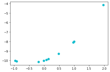
‘c’参数看起来像一个单一的RGB或RGBA数字序列,应避免使用它,因为如果其长度与’x’和’y’匹配,则值映射将具有优先级。如果您确实要为所有点指定相同的RGB或RGBA值,请使用二维数组与一行。
color1 # 一维元组
(0.09019607843137255, 0.7450980392156863, 0.8117647058823529, 1.0)
np.array(color1) # 一维数组,此时对象不分行列;升维前的准备
array([0.09019608, 0.74509804, 0.81176471, 1. ])
np.array(color1).reshape(1, -1) # reshape():改变数组结构,此处用来增维,输入(1, -1)是让行上的维度为1,(-1, 1)是让列上的维度为1# 一行四列
array([[0.09019608, 0.74509804, 0.81176471, 1. ]])
np.array(color1).reshape(-1, 1)# 一列四行
array([[0.09019608],[0.74509804],[0.81176471],[1. ]])
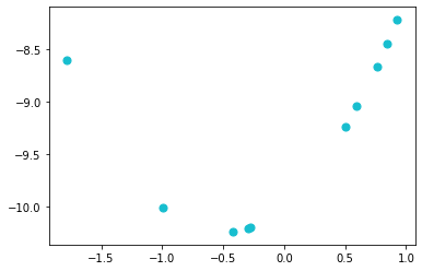
color1 = plt.cm.tab10(5.2)x1 = np.random.randn(10)x2 = x1 + x1**2 - 10plt.scatter(x1, x2, s = 50, c = np.array(color1).reshape(1, -1))
<matplotlib.collections.PathCollection at 0x10fc66ea780>
3. 生成图像
midwest.head()
| PID | county | state | area | poptotal | popdensity | popwhite | popblack | popamerindian | popasian | … | percprof | poppovertyknown | percpovertyknown | percbelowpoverty | percchildbelowpovert | percadultpoverty | percelderlypoverty | inmetro | category | dot_size | |
|---|---|---|---|---|---|---|---|---|---|---|---|---|---|---|---|---|---|---|---|---|---|
| 0 | 561 | ADAMS | IL | 0.052 | 66090 | 1270.961540 | 63917 | 1702 | 98 | 249 | … | 4.355859 | 63628 | 96.274777 | 13.151443 | 18.011717 | 11.009776 | 12.443812 | 0 | AAR | 250.944411 |
| 1 | 562 | ALEXANDER | IL | 0.014 | 10626 | 759.000000 | 7054 | 3496 | 19 | 48 | … | 2.870315 | 10529 | 99.087145 | 32.244278 | 45.826514 | 27.385647 | 25.228976 | 0 | LHR | 185.781260 |
| 2 | 563 | BOND | IL | 0.022 | 14991 | 681.409091 | 14477 | 429 | 35 | 16 | … | 4.488572 | 14235 | 94.956974 | 12.068844 | 14.036061 | 10.852090 | 12.697410 | 0 | AAR | 175.905385 |
| 3 | 564 | BOONE | IL | 0.017 | 30806 | 1812.117650 | 29344 | 127 | 46 | 150 | … | 4.197800 | 30337 | 98.477569 | 7.209019 | 11.179536 | 5.536013 | 6.217047 | 1 | ALU | 319.823487 |
| 4 | 565 | BROWN | IL | 0.018 | 5836 | 324.222222 | 5264 | 547 | 14 | 5 | … | 3.367680 | 4815 | 82.505140 | 13.520249 | 13.022889 | 11.143211 | 19.200000 | 0 | AAR | 130.442161 |
5 rows × 29 columns
方法一
plt.figure(figsize = (16, 10))# 循环次数 = 标签数 = 颜色数 = 需要生成的小数的个数for i in range(len(categories)):plt.scatter(midwest.loc[midwest['category'] == categories[i], 'area'],midwest.loc[midwest['category'] == categories[i], 'poptotal'],s = 20,c = np.array(plt.cm.tab10(i / len(categories))).reshape(1, -1),label = categories[i])plt.legend()
<matplotlib.legend.Legend at 0x10fc670ce10>
方法二
# 列表推导式生成颜色列表,然后用索引将颜色依次取出colors = [plt.cm.tab10(i/float(len(categories) - 1)) for i in range(len(categories))]'''等同于:colors = []for i in range(len(categories)):colors.append(plt.cm.tab10(i/float(len(categories) - 1)))'''plt.figure(figsize = (16, 10))for i in range(len(categories)):plt.scatter(midwest.loc[midwest['category'] == categories[i], 'area'],midwest.loc[midwest['category'] == categories[i], 'poptotal'],s = 20,c = np.array(colors[i]).reshape(1, -1),label = categories[i])plt.legend()
<matplotlib.legend.Legend at 0x10fc6b5df98>
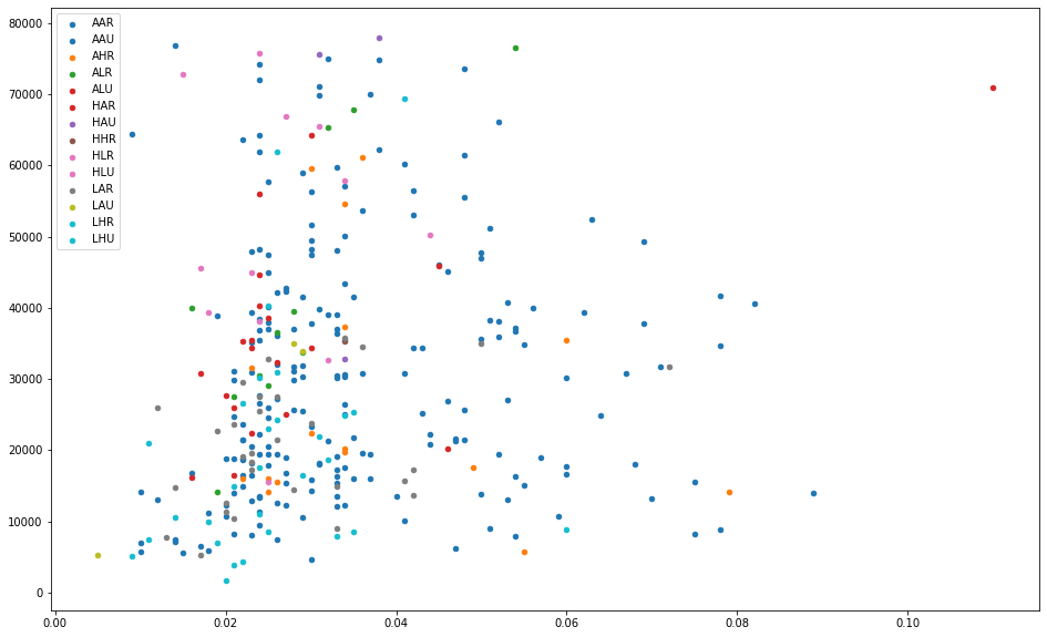
colors # 一个列表,包含14个元组
[(0.12156862745098039, 0.4666666666666667, 0.7058823529411765, 1.0),(0.12156862745098039, 0.4666666666666667, 0.7058823529411765, 1.0),(1.0, 0.4980392156862745, 0.054901960784313725, 1.0),(0.17254901960784313, 0.6274509803921569, 0.17254901960784313, 1.0),(0.8392156862745098, 0.15294117647058825, 0.1568627450980392, 1.0),(0.8392156862745098, 0.15294117647058825, 0.1568627450980392, 1.0),(0.5803921568627451, 0.403921568627451, 0.7411764705882353, 1.0),(0.5490196078431373, 0.33725490196078434, 0.29411764705882354, 1.0),(0.8901960784313725, 0.4666666666666667, 0.7607843137254902, 1.0),(0.8901960784313725, 0.4666666666666667, 0.7607843137254902, 1.0),(0.4980392156862745, 0.4980392156862745, 0.4980392156862745, 1.0),(0.7372549019607844, 0.7411764705882353, 0.13333333333333333, 1.0),(0.09019607843137255, 0.7450980392156863, 0.8117647058823529, 1.0),(0.09019607843137255, 0.7450980392156863, 0.8117647058823529, 1.0)]
参考
# 预设图像的各种属性large = 22; med = 16; small = 12params = {'legend.fontsize': med, # 图例的字体大小'figure.figsize': (16, 10), # 图像的画布大小'axes.labelsize': med, # 标签的字体大小'axes.titlesize': med, # 子图上的标题字体大小'xtick.labelsize': med, # x轴上的标尺的字体大小'ytick.labelsize': med, # y轴上的标尺的字体大小'figure.titlesize': large} # 整个画布的标题字体大小plt.rcParams.update(params) # 设定各种默认风格plt.style.use('seaborn-whitegrid') # 设定整体风格sns.set_style("white") # 设定整体背景风格# Prepare Data# Create as many colors as there are unique midwest['category']categories = np.unique(midwest['category'])colors = [plt.cm.tab10(i/float(len(categories)-1)) for i in range(len(categories))]# Draw Plot for Each Categoryplt.figure(figsize=(16, 10) # 绘图尺寸, dpi= 80 # 图像分辨率, facecolor='w' # 图像的背景颜色,设置为白色,默认也是白色, edgecolor='k' # 图像的边框颜色,设置为黑色,默认也是黑色)for i, category in enumerate(categories):plt.scatter('area', 'poptotal',data=midwest.loc[midwest.category==category, :],s=20, c=np.array(colors[i]).reshape(1, -1), label=str(category))# Decorations# plt.gca() 获取当前子图;若当前没有子图,则创建子图plt.gca().set(xlim=(0.0, 0.12), ylim=(0, 90000), # 控制横纵坐标的范围xlabel='Area', ylabel='Population')plt.xticks(fontsize=12); plt.yticks(fontsize=12)plt.title("Scatterplot of Midwest Area vs Population", fontsize=22)plt.legend(fontsize=12, loc =0)plt.show()
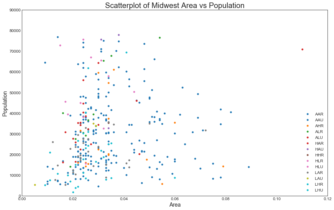
探索数据
异常值
midwest[midwest['area'] > 0.1]
| PID | county | state | area | poptotal | popdensity | popwhite | popblack | popamerindian | popasian | … | percprof | poppovertyknown | percpovertyknown | percbelowpoverty | percchildbelowpovert | percadultpoverty | percelderlypoverty | inmetro | category | dot_size | |
|---|---|---|---|---|---|---|---|---|---|---|---|---|---|---|---|---|---|---|---|---|---|
| 196 | 1248 | MARQUETTE | MI | 0.11 | 70887 | 644.427273 | 68027 | 1170 | 943 | 538 | … | 6.799415 | 66398 | 93.667386 | 12.608814 | 14.26216 | 11.84465 | 12.523891 | 0 | HAR | 171.19829 |
1 rows × 29 columns
标签含义探索
midwest['category'].value_counts()
AAR 186LAR 30LHR 27AAU 21AHR 16ALU 14ALR 11HLU 10HAR 6HAU 3LAU 3LHU 2HLR 2HHR 1Name: category, dtype: int64
midwest['c1'] = midwest['category'].apply(lambda x : x[0])midwest['c2'] = midwest['category'].apply(lambda x : x[1])midwest['c3'] = midwest['category'].apply(lambda x : x[2])midwest.head()
| PID | county | state | area | poptotal | popdensity | popwhite | popblack | popamerindian | popasian | … | percbelowpoverty | percchildbelowpovert | percadultpoverty | percelderlypoverty | inmetro | category | dot_size | c1 | c2 | c3 | |
|---|---|---|---|---|---|---|---|---|---|---|---|---|---|---|---|---|---|---|---|---|---|
| 0 | 561 | ADAMS | IL | 0.052 | 66090 | 1270.961540 | 63917 | 1702 | 98 | 249 | … | 13.151443 | 18.011717 | 11.009776 | 12.443812 | 0 | AAR | 250.944411 | A | A | R |
| 1 | 562 | ALEXANDER | IL | 0.014 | 10626 | 759.000000 | 7054 | 3496 | 19 | 48 | … | 32.244278 | 45.826514 | 27.385647 | 25.228976 | 0 | LHR | 185.781260 | L | H | R |
| 2 | 563 | BOND | IL | 0.022 | 14991 | 681.409091 | 14477 | 429 | 35 | 16 | … | 12.068844 | 14.036061 | 10.852090 | 12.697410 | 0 | AAR | 175.905385 | A | A | R |
| 3 | 564 | BOONE | IL | 0.017 | 30806 | 1812.117650 | 29344 | 127 | 46 | 150 | … | 7.209019 | 11.179536 | 5.536013 | 6.217047 | 1 | ALU | 319.823487 | A | L | U |
| 4 | 565 | BROWN | IL | 0.018 | 5836 | 324.222222 | 5264 | 547 | 14 | 5 | … | 13.520249 | 13.022889 | 11.143211 | 19.200000 | 0 | AAR | 130.442161 | A | A | R |
5 rows × 32 columns
猜测
midwest['c1'].value_counts() # Averaage/High/Low
A 248L 62H 22Name: c1, dtype: int64
midwest['c2'].value_counts() # Averaage/High/Low
A 249H 46L 37Name: c2, dtype: int64
midwest['c3'].value_counts() # Rural/Urban
R 279U 53Name: c3, dtype: int64
机器学习检验猜测:逻辑回归探索数据集
数据预处理
from sklearn.preprocessing import OrdinalEncoder as OEdata = midwest.copy()data.iloc[:, -3:].head()
| c1 | c2 | c3 | |
|---|---|---|---|
| 0 | A | A | R |
| 1 | L | H | R |
| 2 | A | A | R |
| 3 | A | L | U |
| 4 | A | A | R |
data.iloc[:, -3:] = OE().fit_transform(data.iloc[:, -3:])data.iloc[:, -3:].head()# Low = 2# Average = 0# High = 1# Rural = 0# Urban = 1
| c1 | c2 | c3 | |
|---|---|---|---|
| 0 | 0.0 | 0.0 | 0.0 |
| 1 | 2.0 | 1.0 | 0.0 |
| 2 | 0.0 | 0.0 | 0.0 |
| 3 | 0.0 | 2.0 | 1.0 |
| 4 | 0.0 | 0.0 | 0.0 |
data.info()
<class 'pandas.core.frame.DataFrame'>RangeIndex: 332 entries, 0 to 331Data columns (total 32 columns):PID 332 non-null int64county 332 non-null objectstate 332 non-null objectarea 332 non-null float64poptotal 332 non-null int64popdensity 332 non-null float64popwhite 332 non-null int64popblack 332 non-null int64popamerindian 332 non-null int64popasian 332 non-null int64popother 332 non-null int64percwhite 332 non-null float64percblack 332 non-null float64percamerindan 332 non-null float64percasian 332 non-null float64percother 332 non-null float64popadults 332 non-null int64perchsd 332 non-null float64percollege 332 non-null float64percprof 332 non-null float64poppovertyknown 332 non-null int64percpovertyknown 332 non-null float64percbelowpoverty 332 non-null float64percchildbelowpovert 332 non-null float64percadultpoverty 332 non-null float64percelderlypoverty 332 non-null float64inmetro 332 non-null int64category 332 non-null objectdot_size 332 non-null float64c1 332 non-null float64c2 332 non-null float64c3 332 non-null float64dtypes: float64(19), int64(10), object(3)memory usage: 83.1+ KB
data.columns = ["城市ID","郡","州","面积","总人口","人口密度","白人人口","非裔人口","美洲印第安人人口","亚洲人口","其他人种人口","白人所占比例","非裔所占比例","美洲印第安人所占比例","亚洲人所占比例","其他人种比例","成年人口","具有高中文凭的比率","大学文凭比例","有工作的人群比例","已知贫困人口","已知贫困人口的比例","贫困线以下的人的比例","贫困线以下的儿童所占比例","贫困的成年人所占的比例","贫困的老年人所占的比例","是否拥有地铁","标签","点的尺寸","c1","c2","c3"]
# 去掉所有类型为'Object'的列data = data.loc[:, data.dtypes.values != 'O']data.head()
| 城市ID | 面积 | 总人口 | 人口密度 | 白人人口 | 非裔人口 | 美洲印第安人人口 | 亚洲人口 | 其他人种人口 | 白人所占比例 | … | 已知贫困人口的比例 | 贫困线以下的人的比例 | 贫困线以下的儿童所占比例 | 贫困的成年人所占的比例 | 贫困的老年人所占的比例 | 是否拥有地铁 | 点的尺寸 | c1 | c2 | c3 | |
|---|---|---|---|---|---|---|---|---|---|---|---|---|---|---|---|---|---|---|---|---|---|
| 0 | 561 | 0.052 | 66090 | 1270.961540 | 63917 | 1702 | 98 | 249 | 124 | 96.712059 | … | 96.274777 | 13.151443 | 18.011717 | 11.009776 | 12.443812 | 0 | 250.944411 | 0.0 | 0.0 | 0.0 |
| 1 | 562 | 0.014 | 10626 | 759.000000 | 7054 | 3496 | 19 | 48 | 9 | 66.384340 | … | 99.087145 | 32.244278 | 45.826514 | 27.385647 | 25.228976 | 0 | 185.781260 | 2.0 | 1.0 | 0.0 |
| 2 | 563 | 0.022 | 14991 | 681.409091 | 14477 | 429 | 35 | 16 | 34 | 96.571276 | … | 94.956974 | 12.068844 | 14.036061 | 10.852090 | 12.697410 | 0 | 175.905385 | 0.0 | 0.0 | 0.0 |
| 3 | 564 | 0.017 | 30806 | 1812.117650 | 29344 | 127 | 46 | 150 | 1139 | 95.254171 | … | 98.477569 | 7.209019 | 11.179536 | 5.536013 | 6.217047 | 1 | 319.823487 | 0.0 | 2.0 | 1.0 |
| 4 | 565 | 0.018 | 5836 | 324.222222 | 5264 | 547 | 14 | 5 | 6 | 90.198766 | … | 82.505140 | 13.520249 | 13.022889 | 11.143211 | 19.200000 | 0 | 130.442161 | 0.0 | 0.0 | 0.0 |
5 rows × 29 columns
# 将所有整数类型的列转换为浮点数类型for i in range(data.loc[:, data.dtypes.values == 'int64'].shape[1]):data.loc[i, data.dtypes.values == 'int64'] = data.loc[i, data.dtypes.values == 'int64'].apply(lambda x : float(x))
data.info()
<class 'pandas.core.frame.DataFrame'>RangeIndex: 332 entries, 0 to 331Data columns (total 29 columns):城市ID 332 non-null float64面积 332 non-null float64总人口 332 non-null float64人口密度 332 non-null float64白人人口 332 non-null float64非裔人口 332 non-null float64美洲印第安人人口 332 non-null float64亚洲人口 332 non-null float64其他人种人口 332 non-null float64白人所占比例 332 non-null float64非裔所占比例 332 non-null float64美洲印第安人所占比例 332 non-null float64亚洲人所占比例 332 non-null float64其他人种比例 332 non-null float64成年人口 332 non-null float64具有高中文凭的比率 332 non-null float64大学文凭比例 332 non-null float64有工作的人群比例 332 non-null float64已知贫困人口 332 non-null float64已知贫困人口的比例 332 non-null float64贫困线以下的人的比例 332 non-null float64贫困线以下的儿童所占比例 332 non-null float64贫困的成年人所占的比例 332 non-null float64贫困的老年人所占的比例 332 non-null float64是否拥有地铁 332 non-null float64点的尺寸 332 non-null float64c1 332 non-null float64c2 332 non-null float64c3 332 non-null float64dtypes: float64(29)memory usage: 75.3 KB
构建训练集和测试集
- 筛选列作为特征矩阵
- 其他列作为目标向量
- 分训练集和测试集
- 数据标准化(线性模型的核心需求)
X = data.iloc[:, 1:-3]X.head()
| 面积 | 总人口 | 人口密度 | 白人人口 | 非裔人口 | 美洲印第安人人口 | 亚洲人口 | 其他人种人口 | 白人所占比例 | 非裔所占比例 | … | 大学文凭比例 | 有工作的人群比例 | 已知贫困人口 | 已知贫困人口的比例 | 贫困线以下的人的比例 | 贫困线以下的儿童所占比例 | 贫困的成年人所占的比例 | 贫困的老年人所占的比例 | 是否拥有地铁 | 点的尺寸 | |
|---|---|---|---|---|---|---|---|---|---|---|---|---|---|---|---|---|---|---|---|---|---|
| 0 | 0.052 | 66090.0 | 1270.961540 | 63917.0 | 1702.0 | 98.0 | 249.0 | 124.0 | 96.712059 | 2.575276 | … | 19.631392 | 4.355859 | 63628.0 | 96.274777 | 13.151443 | 18.011717 | 11.009776 | 12.443812 | 0.0 | 250.944411 |
| 1 | 0.014 | 10626.0 | 759.000000 | 7054.0 | 3496.0 | 19.0 | 48.0 | 9.0 | 66.384340 | 32.900433 | … | 11.243308 | 2.870315 | 10529.0 | 99.087145 | 32.244278 | 45.826514 | 27.385647 | 25.228976 | 0.0 | 185.781260 |
| 2 | 0.022 | 14991.0 | 681.409091 | 14477.0 | 429.0 | 35.0 | 16.0 | 34.0 | 96.571276 | 2.861717 | … | 17.033819 | 4.488572 | 14235.0 | 94.956974 | 12.068844 | 14.036061 | 10.852090 | 12.697410 | 0.0 | 175.905385 |
| 3 | 0.017 | 30806.0 | 1812.117650 | 29344.0 | 127.0 | 46.0 | 150.0 | 1139.0 | 95.254171 | 0.412257 | … | 17.278954 | 4.197800 | 30337.0 | 98.477569 | 7.209019 | 11.179536 | 5.536013 | 6.217047 | 1.0 | 319.823487 |
| 4 | 0.018 | 5836.0 | 324.222222 | 5264.0 | 547.0 | 14.0 | 5.0 | 6.0 | 90.198766 | 9.372858 | … | 14.475999 | 3.367680 | 4815.0 | 82.505140 | 13.520249 | 13.022889 | 11.143211 | 19.200000 | 0.0 | 130.442161 |
5 rows × 25 columns
Y = data.iloc[:, -3:]Y.head()
| c1 | c2 | c3 | |
|---|---|---|---|
| 0 | 0.0 | 0.0 | 0.0 |
| 1 | 2.0 | 1.0 | 0.0 |
| 2 | 0.0 | 0.0 | 0.0 |
| 3 | 0.0 | 2.0 | 1.0 |
| 4 | 0.0 | 0.0 | 0.0 |
from sklearn.model_selection import train_test_split as TTSXtrain, Xtest, Ytrain, Ytest = TTS(X, Y, test_size = 0.3, random_state = 420)
Xtrain.head()
| 面积 | 总人口 | 人口密度 | 白人人口 | 非裔人口 | 美洲印第安人人口 | 亚洲人口 | 其他人种人口 | 白人所占比例 | 非裔所占比例 | … | 大学文凭比例 | 有工作的人群比例 | 已知贫困人口 | 已知贫困人口的比例 | 贫困线以下的人的比例 | 贫困线以下的儿童所占比例 | 贫困的成年人所占的比例 | 贫困的老年人所占的比例 | 是否拥有地铁 | 点的尺寸 | |
|---|---|---|---|---|---|---|---|---|---|---|---|---|---|---|---|---|---|---|---|---|---|
| 276 | 0.041 | 15682.0 | 382.487805 | 15001.0 | 375.0 | 125.0 | 56.0 | 125.0 | 95.657442 | 2.391277 | … | 12.427492 | 2.390578 | 14534.0 | 92.679505 | 14.435118 | 22.300831 | 13.310056 | 10.186757 | 0.0 | 137.858283 |
| 156 | 0.030 | 23265.0 | 775.500000 | 23127.0 | 2.0 | 50.0 | 41.0 | 45.0 | 99.406834 | 0.008597 | … | 16.583835 | 5.166100 | 22974.0 | 98.749194 | 7.704361 | 8.136567 | 6.168723 | 11.040340 | 0.0 | 187.881402 |
| 35 | 0.036 | 61067.0 | 1696.305560 | 51991.0 | 6342.0 | 109.0 | 2178.0 | 447.0 | 85.137636 | 10.385314 | … | 36.643665 | 14.089892 | 54230.0 | 88.804100 | 28.371750 | 26.392211 | 32.458483 | 13.815301 | 0.0 | 305.082769 |
| 161 | 0.031 | 18185.0 | 586.612903 | 17895.0 | 23.0 | 211.0 | 24.0 | 32.0 | 98.405279 | 0.126478 | … | 19.039803 | 5.014362 | 17942.0 | 98.663734 | 13.214803 | 18.758142 | 12.037542 | 9.681284 | 0.0 | 163.839599 |
| 321 | 0.079 | 14181.0 | 179.506329 | 11962.0 | 18.0 | 2167.0 | 15.0 | 19.0 | 84.352302 | 0.126930 | … | 17.947917 | 4.041667 | 13897.0 | 97.997320 | 20.544002 | 29.073570 | 19.195368 | 14.179318 | 0.0 | 112.022528 |
5 rows × 25 columns
for i in [Xtrain, Xtest, Ytrain, Ytest]:i.index = range(i.shape[0])# Xtrain = Xtrain.reset_index().drop(index) 无法改变原数据Xtrain.head()
| 面积 | 总人口 | 人口密度 | 白人人口 | 非裔人口 | 美洲印第安人人口 | 亚洲人口 | 其他人种人口 | 白人所占比例 | 非裔所占比例 | … | 大学文凭比例 | 有工作的人群比例 | 已知贫困人口 | 已知贫困人口的比例 | 贫困线以下的人的比例 | 贫困线以下的儿童所占比例 | 贫困的成年人所占的比例 | 贫困的老年人所占的比例 | 是否拥有地铁 | 点的尺寸 | |
|---|---|---|---|---|---|---|---|---|---|---|---|---|---|---|---|---|---|---|---|---|---|
| 0 | 0.041 | 15682.0 | 382.487805 | 15001.0 | 375.0 | 125.0 | 56.0 | 125.0 | 95.657442 | 2.391277 | … | 12.427492 | 2.390578 | 14534.0 | 92.679505 | 14.435118 | 22.300831 | 13.310056 | 10.186757 | 0.0 | 137.858283 |
| 1 | 0.030 | 23265.0 | 775.500000 | 23127.0 | 2.0 | 50.0 | 41.0 | 45.0 | 99.406834 | 0.008597 | … | 16.583835 | 5.166100 | 22974.0 | 98.749194 | 7.704361 | 8.136567 | 6.168723 | 11.040340 | 0.0 | 187.881402 |
| 2 | 0.036 | 61067.0 | 1696.305560 | 51991.0 | 6342.0 | 109.0 | 2178.0 | 447.0 | 85.137636 | 10.385314 | … | 36.643665 | 14.089892 | 54230.0 | 88.804100 | 28.371750 | 26.392211 | 32.458483 | 13.815301 | 0.0 | 305.082769 |
| 3 | 0.031 | 18185.0 | 586.612903 | 17895.0 | 23.0 | 211.0 | 24.0 | 32.0 | 98.405279 | 0.126478 | … | 19.039803 | 5.014362 | 17942.0 | 98.663734 | 13.214803 | 18.758142 | 12.037542 | 9.681284 | 0.0 | 163.839599 |
| 4 | 0.079 | 14181.0 | 179.506329 | 11962.0 | 18.0 | 2167.0 | 15.0 | 19.0 | 84.352302 | 0.126930 | … | 17.947917 | 4.041667 | 13897.0 | 97.997320 | 20.544002 | 29.073570 | 19.195368 | 14.179318 | 0.0 | 112.022528 |
5 rows × 25 columns
Xtrain.iloc[:, [*range(23), -1]].head()
| 面积 | 总人口 | 人口密度 | 白人人口 | 非裔人口 | 美洲印第安人人口 | 亚洲人口 | 其他人种人口 | 白人所占比例 | 非裔所占比例 | … | 具有高中文凭的比率 | 大学文凭比例 | 有工作的人群比例 | 已知贫困人口 | 已知贫困人口的比例 | 贫困线以下的人的比例 | 贫困线以下的儿童所占比例 | 贫困的成年人所占的比例 | 贫困的老年人所占的比例 | 点的尺寸 | |
|---|---|---|---|---|---|---|---|---|---|---|---|---|---|---|---|---|---|---|---|---|---|
| 0 | 0.041 | 15682.0 | 382.487805 | 15001.0 | 375.0 | 125.0 | 56.0 | 125.0 | 95.657442 | 2.391277 | … | 66.980137 | 12.427492 | 2.390578 | 14534.0 | 92.679505 | 14.435118 | 22.300831 | 13.310056 | 10.186757 | 137.858283 |
| 1 | 0.030 | 23265.0 | 775.500000 | 23127.0 | 2.0 | 50.0 | 41.0 | 45.0 | 99.406834 | 0.008597 | … | 77.877321 | 16.583835 | 5.166100 | 22974.0 | 98.749194 | 7.704361 | 8.136567 | 6.168723 | 11.040340 | 187.881402 |
| 2 | 0.036 | 61067.0 | 1696.305560 | 51991.0 | 6342.0 | 109.0 | 2178.0 | 447.0 | 85.137636 | 10.385314 | … | 78.767251 | 36.643665 | 14.089892 | 54230.0 | 88.804100 | 28.371750 | 26.392211 | 32.458483 | 13.815301 | 305.082769 |
| 3 | 0.031 | 18185.0 | 586.612903 | 17895.0 | 23.0 | 211.0 | 24.0 | 32.0 | 98.405279 | 0.126478 | … | 76.380796 | 19.039803 | 5.014362 | 17942.0 | 98.663734 | 13.214803 | 18.758142 | 12.037542 | 9.681284 | 163.839599 |
| 4 | 0.079 | 14181.0 | 179.506329 | 11962.0 | 18.0 | 2167.0 | 15.0 | 19.0 | 84.352302 | 0.126930 | … | 73.739583 | 17.947917 | 4.041667 | 13897.0 | 97.997320 | 20.544002 | 29.073570 | 19.195368 | 14.179318 | 112.022528 |
5 rows × 24 columns
# 标准化数据集from sklearn.preprocessing import StandardScalerss = StandardScaler() # 实例化ss = ss.fit(Xtrain.iloc[:, [*range(23), -1]]) # 以训练集为标准的均值和方差Xtrain_ = Xtrain.copy()Xtest_ = Xtest.copy()Xtrain_.iloc[:, [*range(23), -1]] = ss.transform(Xtrain.iloc[:, [*range(23), -1]])Xtest_.iloc[:, [*range(23), -1]] = ss.transform(Xtest.iloc[:, [*range(23), -1]])
Xtrain_.head()
| 面积 | 总人口 | 人口密度 | 白人人口 | 非裔人口 | 美洲印第安人人口 | 亚洲人口 | 其他人种人口 | 白人所占比例 | 非裔所占比例 | … | 大学文凭比例 | 有工作的人群比例 | 已知贫困人口 | 已知贫困人口的比例 | 贫困线以下的人的比例 | 贫困线以下的儿童所占比例 | 贫困的成年人所占的比例 | 贫困的老年人所占的比例 | 是否拥有地铁 | 点的尺寸 | |
|---|---|---|---|---|---|---|---|---|---|---|---|---|---|---|---|---|---|---|---|---|---|
| 0 | 0.616975 | -0.781589 | -0.817515 | -0.806262 | -0.109249 | -0.024001 | -0.298458 | -0.020924 | -0.560519 | 0.359059 | … | -0.879865 | -0.848804 | -0.824188 | -1.455058 | 0.342460 | 0.839258 | 0.428156 | -0.582661 | 0.0 | -0.817515 |
| 1 | -0.141464 | -0.374282 | -0.347133 | -0.350269 | -0.486592 | -0.330845 | -0.368263 | -0.341073 | 0.588691 | -0.457448 | … | -0.002157 | 0.773189 | -0.351151 | 0.550676 | -1.033914 | -1.207832 | -0.982892 | -0.331241 | 0.0 | -0.347133 |
| 2 | 0.272230 | 1.656180 | 0.754945 | 1.269442 | 5.927225 | -0.089461 | 9.576664 | 1.267678 | -3.784901 | 3.098491 | … | 4.233941 | 5.988182 | 1.400655 | -2.735690 | 3.192365 | 1.430564 | 4.211672 | 0.486112 | 0.0 | 0.754945 |
| 3 | -0.072515 | -0.647145 | -0.573205 | -0.643865 | -0.465347 | 0.327847 | -0.447376 | -0.393097 | 0.281709 | -0.417052 | … | 0.516478 | 0.684514 | -0.633180 | 0.522436 | 0.092918 | 0.327251 | 0.176721 | -0.731545 | 0.0 | -0.573205 |
| 4 | 3.237036 | -0.862212 | -1.060456 | -0.976797 | -0.470405 | 8.330347 | -0.489259 | -0.445122 | -4.025610 | -0.416897 | … | 0.285901 | 0.116079 | -0.859890 | 0.302219 | 1.591667 | 1.818087 | 1.591028 | 0.593332 | 0.0 | -1.060456 |
5 rows × 25 columns
from sklearn.linear_model import LogisticRegression as logiRimport pandas as pdfor i in range(3): # c1,c2,c3分别建模# 实例化:logi = logiR(solver = 'newton-cg' # 本例用牛顿法结果更准确, max_iter = 100**20 # 使用牛顿法所需要的迭代次数, multi_class = 'multinomial' # 由于c1和c2是三分类(L/A/H))# 开始建模:logi.fit(Xtrain_, Ytrain.iloc[:, i].ravel())print(Y.columns[i])print('\tTrain:{}'.format(logi.score(Xtrain_, Ytrain.iloc[:, i].ravel()))) # 模型的学习能力,以准确率衡量print('\tTest:{}'.format(logi.score(Xtest_, Ytest.iloc[:, i].ravel()))) # 模型的泛化能力coeff = pd.DataFrame(logi.coef_).Tif i != 2:coeff['mean'] = abs(coeff).mean(axis = 1)coeff['name'] = Xtrain.columnscoeff.columns = ['Average', 'High', 'Low', 'mean', 'name']coeff = coeff.sort_values(by = 'mean', ascending = False).head()else:coeff['name'] = Xtrain.columnscoeff.columns = ['coef', 'name']coeff = coeff.sort_values(by = 'coef', ascending = False).head()print(coeff)print('\t')
c1Train:0.9956896551724138Test:0.97Average High Low mean name14 1.274035 2.189743 -3.463778 2.309186 具有高中文凭的比率15 -0.656186 1.390281 -0.734095 0.926854 大学文凭比例16 -0.363926 0.899042 -0.535116 0.599361 有工作的人群比例21 0.180958 -0.662631 0.481673 0.441754 贫困的成年人所占的比例19 0.231073 -0.534413 0.303341 0.356275 贫困线以下的人的比例c2Train:0.978448275862069Test:0.97Average High Low mean name20 0.248239 1.652407 -1.900646 1.267097 贫困线以下的儿童所占比例21 -0.249106 1.694901 -1.445795 1.129934 贫困的成年人所占的比例19 0.054842 1.639717 -1.694559 1.129706 贫困线以下的人的比例22 -0.105854 0.797378 -0.691524 0.531585 贫困的老年人所占的比例12 -0.552268 0.258467 0.293801 0.368178 其他人种比例c3Train:1.0Test:1.0coef name23 2.981752 是否拥有地铁3 0.104570 白人人口17 0.104304 已知贫困人口1 0.096218 总人口8 0.072634 白人所占比例
mpy.flatten() 与 numpy.ravel()的区别
- 要实现的功能是一致的(将多维数组降位一维)
- 于返回拷贝(copy)还是返回视图(view)
- py.flatten()返回一份拷贝,对拷贝所做的修改不会影响(reflects)原始矩阵
- py.ravel()返回的是视图,会影响原始矩阵
# 实际上不用.ravel()降维也可以。以 i = 0 为例:from sklearn.linear_model import LogisticRegression as logiRimport pandas as pd# 实例化:logi = logiR(solver = 'newton-cg' # 本例用牛顿法结果更准确, max_iter = 100 ** 20 # 使用牛顿法所需要的迭代次数, multi_class = 'multinomial' # 由于本例是三分类(A/H/L))# 开始建模:logi.fit(Xtrain_, Ytrain.iloc[:, 0])print(Y.columns[0])print('\tTrain:{}'.format(logi.score(Xtrain_, Ytrain.iloc[:, 0]))) # 模型的学习能力print('\tTest:{}'.format(logi.score(Xtest_, Ytest.iloc[:, 0]))) # 模型的泛化能力print(logi.coef_.shape) # 25个特征;三分类(L/A/H)一对一:L vs A, L vs H, A vs H
c1Train:0.9956896551724138Test:0.97(3, 25)
解读
midwest['category'].value_counts()
AAR 186LAR 30LHR 27AAU 21AHR 16ALU 14ALR 11HLU 10HAR 6HAU 3LAU 3LHU 2HLR 2HHR 1Name: category, dtype: int64
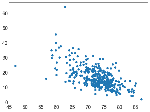
plt.figure(figsize = (8, 6))plt.scatter(data['具有高中文凭的比率'], data['贫困线以下的儿童所占比例'])
<matplotlib.collections.PathCollection at 0x10fc7943dd8>
plt.figure(figsize = (8, 6))categories = np.unique(midwest['category'])colors = [plt.cm.tab10(i/float(len(categories)-1)) for i in range(len(categories))]for i, category in enumerate(categories):plt.scatter('area', 'poptotal',data=midwest.loc[midwest.category==category, :],s=20, c=np.array(colors[i]).reshape(1, -1),label=str(category))plt.legend(fontsize = 12)
<matplotlib.legend.Legend at 0x10fc8aca9e8>

- 中西部大部分地区教育情况和贫困情况处于平均水平
- 蓝绿色的数据点代表教育水平低和贫困水平高,主要分布在图的左下且较为集中,人少地方也小,符合预期
- 有蓝绿色的数据点位于图的右上,人多且穷,需要重点观察,可以提取出来深入研究
- 假设LH的乡村多于LH的城市
- 浅粉色的数据点代表教育水平高和贫困水平低,在图上的分布显示地狭人稠
- 假设HL的城市多余HL的乡村
- 异常点:教育水平高,贫困水平也高(读书无用);教育水平低,贫困水平也低(读书更没用了)
- 图例上只有HHR,没有HHU
- 图例上没有LLU和LLR
由于只取了十种颜色(tab10),所以省略了一些信息,需要更多的颜色显示图例,才能看出城市(U)和乡村(R)的区别
plt.figure(figsize = (10, 8))categories = np.unique(midwest['category'])colors = [plt.cm.tab10(i/float(len(categories)-1)) for i in range(len(categories))]for i, category in enumerate(categories):plt.scatter('area', 'poptotal',data=midwest.loc[midwest.category==category, :],s=20, c=np.array(colors[i]).reshape(1, -1),label=str(category))plt.scatter('area', 'poptotal',data=midwest.loc[midwest.category == 'LHU', :],s = 150,facecolors = 'None', # 点的填充颜色,None代表透明edgecolors = 'red', # 点的边框颜色label = 'Selected Urban')plt.scatter('area', 'poptotal',data=midwest.loc[midwest.category == 'LHR', :],s = 150,facecolors = 'None', # 点的填充颜色,None代表透明edgecolors = 'y', # 点的边框颜色label = 'Selected Rural')plt.legend(fontsize = 12)
<matplotlib.legend.Legend at 0x10fca1ebd30>
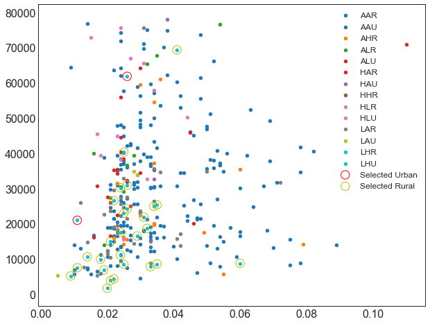
教育水平低且贫困水平高的地区,多数是乡村;核心问题是乡村
plt.figure(figsize = (10, 8))categories = np.unique(midwest['category'])colors = [plt.cm.tab10(i/float(len(categories)-1)) for i in range(len(categories))]for i, category in enumerate(categories):plt.scatter('area', 'poptotal',data=midwest.loc[midwest.category==category, :],s=20, c=np.array(colors[i]).reshape(1, -1),label=str(category))plt.scatter('area', 'poptotal',data=midwest.loc[midwest.category == 'HLU', :],s = 150,facecolors = 'None', # 点的填充颜色,None代表透明edgecolors = 'red', # 点的边框颜色label = 'Selected Urban')plt.scatter('area', 'poptotal',data=midwest.loc[midwest.category == 'HLR', :],s = 150,facecolors = 'None', # 点的填充颜色,None代表透明edgecolors = 'y', # 点的边框颜色label = 'Selected Rural')plt.legend(fontsize = 12)
<matplotlib.legend.Legend at 0x10fca296438>
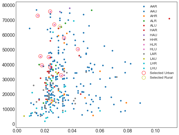
plt.figure(figsize = (10, 8))categories = np.unique(midwest['category'])colors = [plt.cm.tab10(i/float(len(categories)-1)) for i in range(len(categories))]for i, category in enumerate(categories):plt.scatter('area', 'poptotal',data=midwest.loc[midwest.category==category, :],s=20, c=np.array(colors[i]).reshape(1, -1),label=str(category))plt.scatter('area', 'poptotal',data=midwest.loc[midwest.category == 'HHR', :],s = 150,facecolors = 'None', # 点的填充颜色,None代表透明edgecolors = 'red', # 点的边框颜色label = 'Selected Urban')plt.legend(fontsize = 12)
<matplotlib.legend.Legend at 0x10fca31b668>
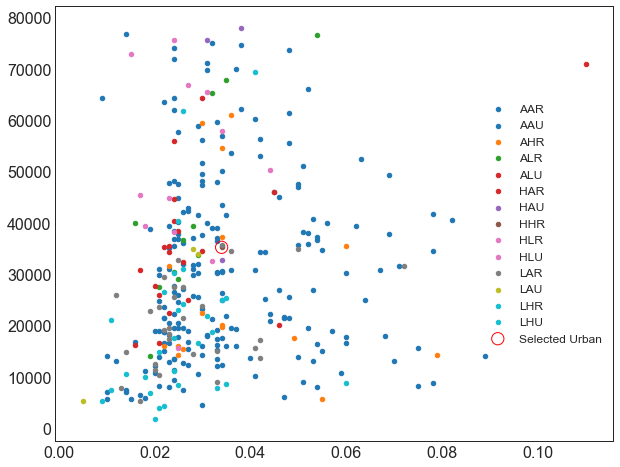
只有一个点教育水平高,贫困水平也高
midwest[midwest['category'] == 'HHR']
| PID | county | state | area | poptotal | popdensity | popwhite | popblack | popamerindian | popasian | … | percbelowpoverty | percchildbelowpovert | percadultpoverty | percelderlypoverty | inmetro | category | dot_size | c1 | c2 | c3 | |
|---|---|---|---|---|---|---|---|---|---|---|---|---|---|---|---|---|---|---|---|---|---|
| 47 | 615 | MCDONOUGH | IL | 0.034 | 35244 | 1036.58824 | 32992 | 1254 | 65 | 802 | … | 19.05208 | 16.009317 | 22.403382 | 12.884384 | 0 | HHR | 221.113063 | H | H | R |
1 rows × 32 columns

若有收获,就点个赞吧
0 人点赞


